KYNEX Bulletin
June 2008
We are pleased
to announce the release of support for volatility surfaces for the pricing of
convertible securities and equity options. Specifying a volatility surface that
captures your view of the implied volatility in the market will result in the
following benefits:
-
Precise control
over the valuation of equity options and the convertible securities.
-
Obtain a Delta
profile for hedging that reflects your view of the relationship between spot
prices, strikes, expirations and implied volatilities.
We describe how
to create, edit and save a volatility surface later
in this document, with an explanation of all of the input fields, and we
also offer several general comments on the specification
of volatility surfaces in conjunction with our existing infrastructure (e.g.
the New Issue Analytic, the Sensitivity screen, etc.). We also emphasize here
that you could continue to value equity derivatives without a volatility
surface, i.e. flat volatility. We analyzed several instruments (equity options
and convertibles) with flat volatilities and volatility surfaces, and we present a summary of our observations below:
·
The effect of
the skew in the volatility surface on the valuation is more pronounced as the
time to expiration increases. This is especially true for long dated equity
options and long call protected convertible securities that have been coming to
market in the past year. We strongly recommend the specification of volatility
surfaces for valuing convertible securities with over three years of call
protection.
·
Volatility
surface is a better way to capture skew in valuing mandatory convertibles. If
the mandatory convertible has structural features such as calls, and one-to-one
upside participation that make a simple decomposition difficult, volatility
surfaces is the only way to capture the skew in valuation.
·
Volatility
surface is a better way to value convertibles with variable conversion ratio
(aka embedded warrants) features. You can specify a surface that captures the
appropriate volatilities for the complex set of options that get embedded into
a convertible security with the variable conversion ratio feature.
Briefly, the input
volatility surface consists of a set of implied volatilities, with their
associated strikes and maturities. (The model will interpolate or extrapolate
the surface as required, for valuing equity derivatives.) Since convertible
bonds are valued on a risky basis, the inputs are treated as risky implied volatilities. We include a
discussion of the concept of risky and risk-free implied volatilities in the
following section.
The general
“volatility surface” referred to by market practitioners is in fact a surface
of implied volatilities. The new functionality allows you to input a set of
implied volatilities, for selected expirations and strikes (as well as a time
factor to grow or decrease the implied volatility beyond the last input
expiration). The valuation model internally calculates a so-called “local
volatility” surface, for pricing the equity derivative such as an equity option
or a convertible security. We have implemented the well-known Dupire formula [B. Dupire, “Pricing and hedging with smiles”
Proc.
Another point to
note is that for exchange-traded listed equity options, the implied
volatilities are calculated by valuing the options on a risk-free basis. One
can call this a “risk-free” implied volatility (risk-free in the sense of
having no default and counter-party risk). However, a risky basis is more
appropriate for the valuation of convertibles, because the option embedded in a
convertible is written by the issuer (not an exchange), and one must
take into account the possibility of default by the issuer. The concept of risky and risk-free implied volatilities is discussed in
more detail in the companion article. Temporarily setting aside the put
and call features of a convertible, a common visualization of a convertible is a
straight bond (paying periodic coupons and principal at maturity) and a call
option on the underlying stock. The straight bond is treated as risky and the
call option is treated as risk-free. This view point suffers from the
deficiency that it is assumed that the bond floor will hold as parity approaches
zero. However, at a zero stock price, the issuer is in default (bankrupt) and
therefore does not have the ability to honor the principal redemption amount of
the bond. A more fundamental way to visualize a convertible is to treat it as a
stock plus a put option (plus coupons). As the stock price goes to zero, the
put goes more in the money, but the issuer’s ability to honor the put becomes
more and more questionable. Hence the implied volatility of a convertible is
effectively that of a risky put
option, i.e. a risky implied volatility.
Another way to state this is the implied volatility of a convertible is the
volatility an options broker would be willing to pay for a put whose ability to
collect when it gets in-the-money is tied to the credit worthiness of the
issuer.
However, note
that the visualization of a convertible as a straight bond plus call option, or
as a stock plus put option, is only approximate. The option embedded in a
convertible does not have a fixed strike or expiration. The effective strike of
the embedded option is a function of the time to maturity. An approximate
measure of the expiration of the embedded option is the median life of the
convertible. Hence when we speak of a “risky put option” or a “risk-free call
option” we are not implying that a
rigorous separation of the option from the convertible bond exists. Overall,
the above ideas lead to the following two points of view when pricing a
convertible using an implied volatility surface (and a third for
exchange-listed equity options):
·
You can specify
a surface of risky implied volatilities. This will value the embedded risky put
in the convertible. In particular, the risky implied volatility should decrease
to zero as the stock price decreases to zero, which indicates the decreasing
probability that the risky put will be honored as the stock price declines. An
investor is less willing to pay for implied volatility for a security which is
unlikely to be honored. Conversely, an investor would be willing to pay a
higher implied volatility for a security with a greater likelihood of a
positive payoff; hence the risky implied volatility increases as the stock
price increases. However, at high parity,
the embedded put is way out of the money (and has negligible Gamma), and once
again an investor would pay a lower implied volatility. Hence, overall, a
surface of risky implied volatilities has a peak as the parity level increases from
low to high values.
·
You can specify
a surface of risk-free implied volatilities (for example, obtained or extrapolated
from the listed options market). In this case you should switch on the
bankruptcy mode (with an appropriately chosen decay factor that captures the
relationship between stock prices and credit spreads) to model the fact that the
bond floor is not guaranteed to hold as parity approaches zero. However, it is
inconsistent to employ a surface of risk-free implied volatilities for a
convertible, without modeling the fact that the bond floor will not hold at
zero parity. In the post-1987 era, the implied volatility surfaces of listed
options (which are risk-free implied volatilities) typically have a negative skew, i.e. the implied
volatility decreases monotonically as the strike level increases.
·
For valuing exchange-listed
equity options, a surface of risk-free implied volatilities is appropriate.
There is no concept of a bankruptcy mode for valuing equity options because
there is no counter-party risk.
To illustrate
these ideas, we display examples of the valuation of equity options using a surface
of risk-free implied volatilities, and convertible bonds using both a surface
of (i) risky implied volatilities and (ii) risk-free implied volatilities with
bankruptcy mode. For the equity option, we select the AG 60 strike Jan 2010
call and put options. For convertibles, for simplicity we consider two bullet
bonds with maturities of at least 5 years. We value the CAI bullet bond
maturing in May 2014 using a risky implied volatility surface, and we value the
NDAQ bullet bond maturating in August 2013 using a risk-free implied volatility
surface, with bankruptcy mode. We summarize our overall findings as follows.
·
We analyzed the
valuation of the fair value and Delta as a function of the stock price, for a
fixed trade date. Next we analyzed the valuation as a function of the trade
date (i.e. time to maturity), for a fixed stock price. We refer to the change
in the implied volatility with the strike level as volatility skew or curvature
(for a risky implied surface with a downward curvature).
o
For equity
options valued using a risk-free implied volatility surface with a negative
skew, the valuation basically follows what one would expect.
§
When sweeping
the stock price the fair value is higher using a volatility surface at low
stock prices (compared to valuing with a flat volatility) and lower at high stock
prices. The Delta is lower at moderate stock prices, and is higher at very low
and very high stock prices.
§
When varying the
trade date (time to expiration), the difference in valuation (for the fair
value) is approximately linear to time-to-expiration, and also approximately
linear in the volatility skew.
o
For convertibles
valued using a risky volatility surface with a negative curvature, the
valuation is more complicated.
§
When sweeping
the stock price the fair value is lower using a volatility surface (compared to
valuing with a flat volatility). This can be understood because of the negative
curvature; the volatility in the surface is lower than the flat assumed
volatility.
§
However, the Delta
displays a complicated behavior, and can be either higher or lower than the Delta
obtained using a flat volatility, depending on the stock price level. The
precise behavior of the Delta is a function of several inputs such as credit spread;
borrow cost, dividends on the stock, etc.
§
When varying the
trade date (time to expiration), the difference in valuation (for the fair
value) is highly nonlinear along time-to-expiration and also nonlinear along
volatility-skew.
o
For convertibles
valued using a risk-free volatility surface with a negative curvature, and the
bankruptcy mode, the valuation is also more complicated.
§
When sweeping
the stock price the fair value is usually but not always lower than with a
volatility surface (compared to valuing with a flat volatility). The precise
behavior depends on many factors.
§
However, the Delta
displays a behavior similar to that of equity options. The Delta is lower at
moderate parity levels, and is higher at very low and very high parity.
§
When varying the
trade date (time to expiration), the difference in valuation (for the fair
value) is approximately linear along time-to-expiration, and also approximately
linear along volatility-skew.
·
In addition to a
volatility skew or curvature, we also allow you to input a time factor, so that
the implied volatilities will grow (or decay) at a specified rate. For example
a time factor of -1 means the volatilities decrease to 99% of their original
values after 1 year. We also analyzed the valuations of equity options and
convertible bonds as a function of time factor decay of the implied
volatilities.
o
We found that in
all cases, when valuing with a volatility surface with a time factor, the
difference in valuation (for the fair value) is approximately linear along time-to-expiration,
and also approximately linear along time-factor.
We now present
more detailed descriptions of our valuations. We begin with the equity options.
The implied volatility surface is presented in Fig. 1. The
at-the-money implied volatility of 44.5 was taken from the 60 strike Jan 2010 listed
options. We also input two other strikes of 40 and 80, and a negative skew of 3
volatility points (i.e. implied volatilities of 47.5 and 41.5, respectively.)
We present the relationship between fair value and stock price for a Jan 2010
call option, in Fig. 2. The blue curve is the valuation
using a flat assumed volatility of 44.5 (the at-the-money implied volatility),
and the pink curve is the valuation obtained using the implied volatility surface.
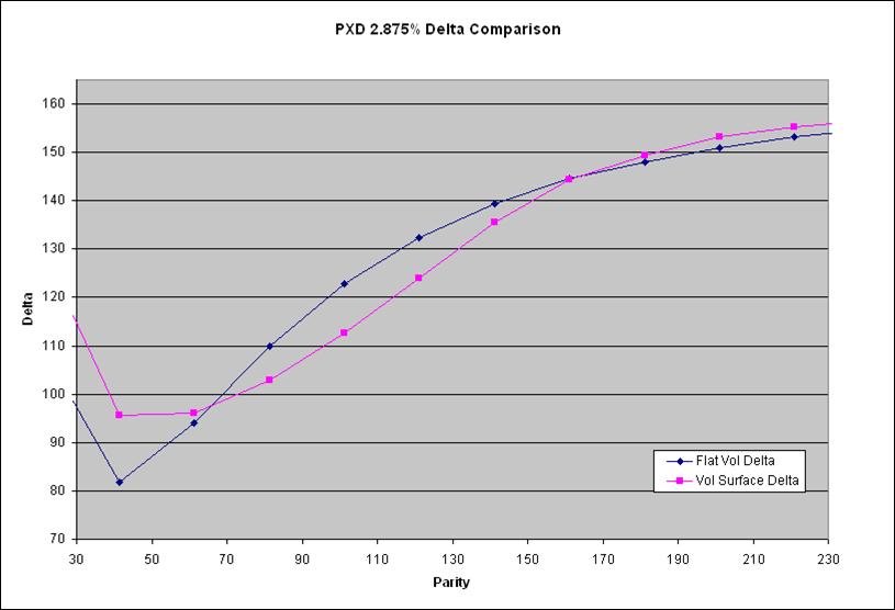
In. Fig. 3, we present the relationship between Delta and
stock price for the same option. As before, the blue and pink curves are the
valuations using a flat assumed volatility and an implied volatility surface,
respectively. We note the following general observations.
·
The graph of the
fair value (Fig. 2) displays a
“crossover” behavior. The valuation using an implied volatility surface is
higher (than the valuation using a flat assumed volatility) at low stock prices,
and is lower at high stock prices. This behavior can be understood because of
the negative skew of the implied volatility, because the implied volatility is
higher at low stock prices and lower at high stock prices. There is no simple formula for the
location of the crossover point, in general.
·
The graph of the
Delta (Fig. 3) has two crossover points. The valuation
using an implied volatility surface is higher (than the valuation using a flat
assumed volatility) at low and high stock prices, and is lower at moderate stock
prices. This behavior can also be understood because of the negative skew of
the implied volatility.
o
At moderate stock
prices, the fair value crosses from a higher to a lower valuation (compared to
a flat assumed volatility), and so overall has a lower slope. Hence the Delta
is lower at moderate stock prices.
o
At high stock
prices, the fair value approaches intrinsic value more rapidly (compared to
valuation using a flat assumed volatility), so the Delta approaches 100 more
rapidly. Hence the Delta is higher using an implied volatility surface.
o
Conversely, at
low stock prices the fair value is higher (compared to valuation using a flat
assumed volatility), but we also know that the fair value equals zero at a
stock price of zero. Hence again the Delta is higher using an implied
volatility surface.
o
As with the
graph for the fair value, there is no simple formula for the locations of the
crossover points.
·
For put options,
we consider the AG 60 strike Jan 2010 put. We display a graph of the fair value
vs. stock price in Fig. 4 and a graph of Delta vs. stock
price in Fig. 5. As before, the blue and pink curves show
the valuation using a flat assumed volatility and an implied volatility
surface, respectively.
o
As for a call
option, the fair value graph shows a crossover where the valuation using an
implied volatility surface is higher at low stock prices and low at higher
stock prices.
o
For the graph of
Delta, the crossover behavior is as follows: at moderate stock prices the Delta
is more negative (higher absolute value), whereas at low and high stock prices,
the Delta is less negative (smaller absolute value).
Another way to
analyze the data is to graph the valuation as a function of the time to
expiration, i.e. to sweep the trade date. In Fig. 6, we
plot a graph of the fair value vs. the trade date, for a fixed stock price
S=40. We display multiple curves, for an implied volatility skew of 0, 1.5, 3.0
and 4.5, respectively (the skew of zero is a flat assumed volatility). The
differences in the valuations are approximately linear in the time to
expiration and also approximately linear in the skew. This is only an approximate
relation, because it is known theoretically that as the time to expiration
increases to infinity (perpetual options), the fair value approaches an
asymptotic limit. Hence the differences shown in Fig. 6 cannot
grow forever but must approach asymptotic limits. However, for moderate skews
and times to expiration (a few years), the above linear relationship is
approximately valid.
There is also
another type of implied volatility surface to consider, i.e. a time structure
(as opposed to an implied volatility skew). We display a second implied
volatility surface in Fig. 7. The time factor is -1 which
means the implied volatilities decay by 1% per year. To simplify the analysis,
we set the skew to zero, so the implied volatility is 44.5 at all the strike
levels. Hence after 1 year, the extrapolated implied volatilities will be![]() . In Fig. 8, we display a graph of the fair
value vs. the trade date, for a fixed stock price S=40. We display multiple
curves, for time factors of 0, –1, –2 and –3, respectively (the time factor of
zero is a flat assumed volatility). The valuation is very similar to Fig. 6, except now a more negative time factor yields a
smaller fair value. The differences in the valuations are approximately linear
in the time factor and actually slightly faster than linear in the time to
expiration.
. In Fig. 8, we display a graph of the fair
value vs. the trade date, for a fixed stock price S=40. We display multiple
curves, for time factors of 0, –1, –2 and –3, respectively (the time factor of
zero is a flat assumed volatility). The valuation is very similar to Fig. 6, except now a more negative time factor yields a
smaller fair value. The differences in the valuations are approximately linear
in the time factor and actually slightly faster than linear in the time to
expiration.
The valuations
for other call and put options are basically similar. To simplify our analysis,
we have demonstrated valuations using either an implied volatility skew or a
time factor for implied volatility decay. However, in general you would specify
both a skew and a time factor together. The effect of a negative time factor changes
the valuation downwards at all stock price levels. The effect of volatility
skew is minimal near the crossover point, and has an opposite effect on the
valuation on either side of the crossover point. However, there is no simple
formula to determine where the crossover point will be located.
We now analyze
the valuation of convertible bonds. We consider the
·
We display a
graph of the fair value vs. parity in Fig. 10. As with
the valuation of the equity options above, the blue curve is the valuation
using a flat assumed volatility (i.e., the 100% strike implied volatility of 45),
and the pink curve is the valuation obtained using the implied volatility
surface. The fair value using an implied volatility surface is always lower
than the fair value using a flat assumed volatility. This is expected because
the volatility from the surface is always lower than the flat assumed
volatility of 45. Note that the asymptotic limits at zero and infinite parity
are independent of the volatility. Hence the bond floor is the same,
independent of the volatility. At very high parity, both valuations also
converge to the same limit.
·
In. Fig. 11, we display a graph of Delta vs. parity. However, we
display three curves. The blue curve
is the valuation using the flat assumed volatility of 45, and the pink curve is
the valuation using an implied volatility surface with a curvature of 3 points.
The yellow curve is the valuation using implied volatility surface with a
curvature of 1 point. Unlike the corresponding graph for equity options, the
crossover behavior for the Delta of a convertible is much more complicated. The
Delta is initially lower at low parity, and is higher at moderate parity, and
there is a second crossover point at a parity of about 90. However, for a
curvature of 3 points, there is a third
crossover point at a very high parity of about 160. Basically, the option
embedded in a convertible cannot be expressed as a simple equity option.
·
In. Fig. 12, we also display a graph of Delta vs. parity, but we
set the trade date forward to
Next, we plot
valuations of the convertible as a function of the trade date, i.e. the time to
maturity. In Fig. 13, we display graph of the fair value
vs. trade date, for curvature values of 0, 1, 2 and 3 points (zero curvature is
same as a flat volatility specification). The curves are respectively blue, pink, yellow,
and light blue. The stock price was set to 60 in the valuations. Unlike the
case for equity options, the difference in valuations for a convertible is
highly nonlinear in the time to expiration, and also in the curvature of the implied
volatility.
·
In general, as
the time to maturity increases, the fair value using an implied volatility
surface stays close to that using a flat assumed volatility, and then diverges
rapidly in a very nonlinear manner. The difference in valuation is small for
times less than one year to maturity (approximately) but grows very fast as the
time to maturity increases beyond that value.
·
For a curvature
of 1 point, the fair value (pink curve) remains fairly close to the valuation
using a flat assumed volatility (blue curve) for all the trade dates in the graph.
However, there are significant differences in valuation for curvatures of 2 and
3 points. The difference in valuation increases nonlinearly with an increase of
curvature.
Next, we value
the convertible bond using an implied volatility surface with a time factor for
the volatility decay. We display the implied volatility surface in Fig. 14. The time factor is –1, which again means the
implied volatilities decay by 1% per year. We set the curvature to zero, so the
implied volatility is 45 at all the strike levels. We set the stock price to
60. In Fig. 15, we display a graph of the fair value vs.
the trade date, for time factors of 0, –1, –2 and –3, respectively (the time
factor of zero is a flat assumed volatility). The curves are blue, pink, yellow and light
blue, respectively.
·
As expected, a
more negative time factor yields a lower fair value.
·
In contrast to
the previous graph (Fig. 13), as the time factor is
varied the difference in valuation is approximately linear in the time to
expiration, and is also approximately linear in the time factor.
·
The magnitude of
the differences in valuation, between Fig. 13 (change of
curvature) and Fig. 15 (change of time factor), are
approximately comparable. In general, you would input an implied volatility
surface using a term structure of curvatures and a time factor.
The valuations
for other convertibles are similar. There are quantitative differences if the
bond has call and put provisions. There are also differences of detail due to dividend
protection, because the changes the conversion ratio depend on the stock price
history, i.e. the volatility.
Next, we analyze
the valuation of convertible bonds using a risk-free implied volatility surface
and the bankruptcy mode. We consider the
·
We display a
graph of the fair value vs. parity in Fig. 17. We display
three curves, where the blue, pink and yellow curves are for skew values of 0,
3 and 6, respectively. (The skew of zero is same as flat assumed volatility of
37.) As expected because of the bankruptcy mode, the fair value decreases to
zero at a parity of zero.
o
The valuation
using a skew of 6 (yellow curve) is always lower than the valuation using a
flat volatility (blue curve). There is no crossover behavior as with equity
options.
o
However, for a
skew of 3 points (pink curve), in an interval of parity from about 55 to 85,
the valuation using a volatility surface is slightly higher than the valuation
using a flat volatility.
o
One can
understand the above results as follows. At high parity, the negative slope of
the volatility surface causes the convertible to be valued with lower
volatility, hence a smaller fair value. At low parity, one expects the
converse, but there is a competing effect from the bankruptcy mode. The higher
volatility at low parity makes it easier for the stock to reach lower levels,
where the credit spread (i.e. the discounting of cashflows) is larger, which in
turn reduces the fair value. Hence there is a balance between two competing effects,
and it is not obvious what will happen to the overall valuation.
·
Next, we display
a graph of the Delta vs. parity in Fig. 18. We again
display three curves, where the blue, pink and yellow curves are for skew
values of 0, 3 and 6, respectively, and the skew of zero assumed a flat volatility
of 37. Also as expected because of the bankruptcy mode, the Delta increases to
infinity at a parity of zero.
o
As was the case
with equity options, the Delta displays two crossover points. At moderate
parity, the Delta is lower when the convertible is valued using a volatility
surface. Also, the Delta (using a volatility surface) is higher at low and high
parity. The locations of the crossover points depend on many factors and are
not described by a simple formula.
Next, we plot
valuations of the convertible as a function of the trade date, i.e. the time to
maturity. In Fig. 19, we display graph of the fair value
vs. trade date, for skew values of 0, 1, 2 and 3 points. (The valuation for
zero is same as flat assumed volatility.) The curves are respectively blue,
pink and yellow, respectively. The stock price was set to 33.15 in the
valuations. Unlike the case for equity options, the difference in valuations
for a convertible in completely nonlinear. No simple conclusion can be drawn.
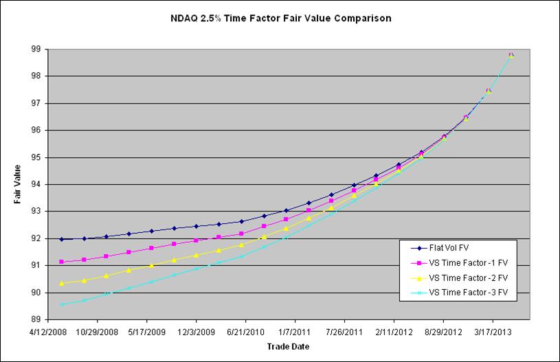
Next, we value
the convertible using an implied volatility surface with time factor decay. The
implied volatility surface is shown in Fig. 20. We set
the implied volatilities to 37 at all strike levels, so the skew is zero. We
set the stock price to 33.15. In Fig. 21, we display a
graph of the fair value vs. the trade date, for time factors of 0, –1, –2 and
–3, respectively (the time factor of zero is a flat assumed volatility). The
curves are blue, pink, yellow and light blue, respectively.
·
As expected, a
more negative time factor yields a lower fair value.
·
Similar to
equity options, the differences in valuation are approximately linear in the
time to expiration, and also approximately linear in the time factor.
Fig. 1 Implied Volatility Surface for AG Showing Volatility Skew
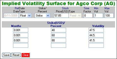
Fig. 2 AG 60 Jan 2010 Call Fair Value vs. Stock Price
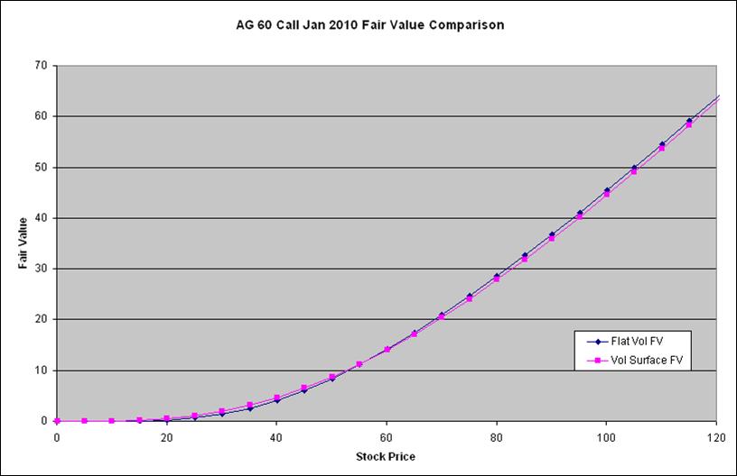
Fig. 3 AG 60 Jan 2010 Call Delta vs. Stock Price
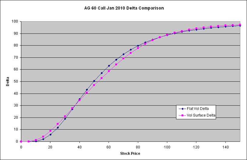
Fig. 4 AG 60 Jan 2010 Put Fair Value vs. Stock Price
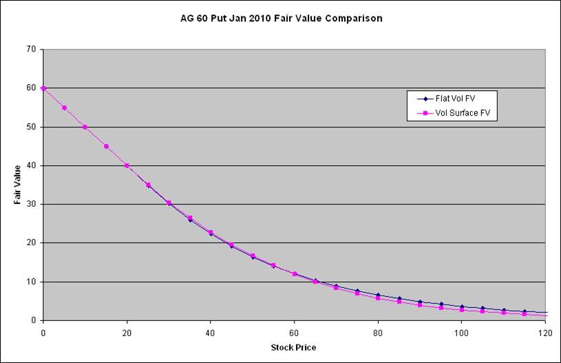
Fig. 5 AG 60 Jan 2010 Put Delta vs. Stock Price
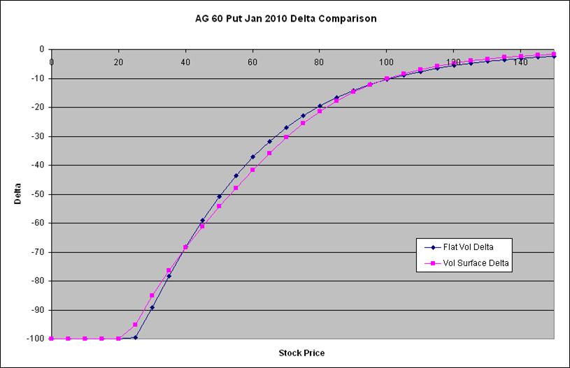
Fig. 6 AG 60 Jan 2010 Call Fair value Time Scan (with fixed stock
price=40) for Multiple Volatility Skews
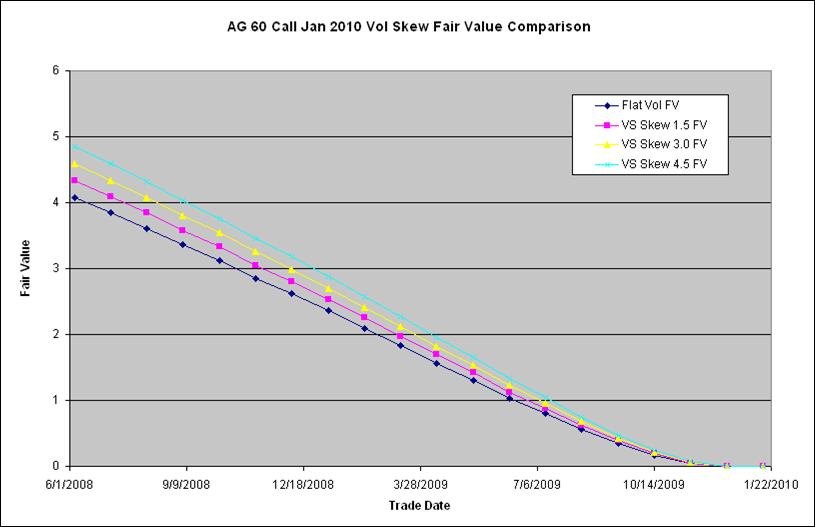
Fig. 7 AG Implied Volatility Surface with Time Factor

Fig. 8 AG 60 Jan 2010 Call Fair Value Time Scan (with fixed stock
price=40) for Multiple Time Factors
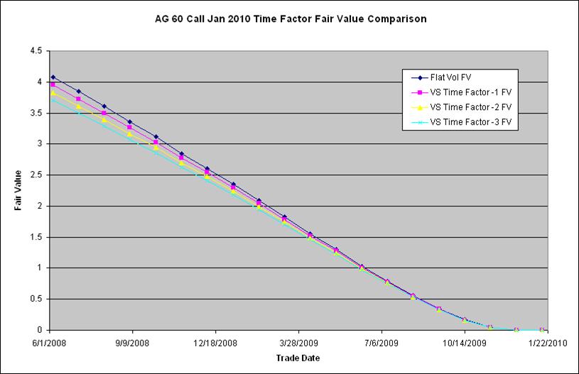
Fig. 9
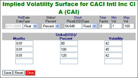
Fig. 10
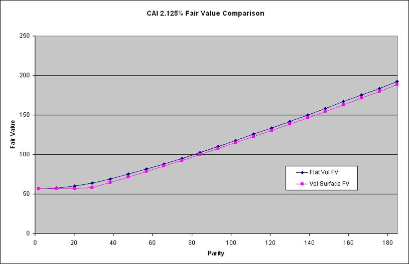
Fig. 11
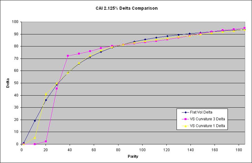
Fig. 12
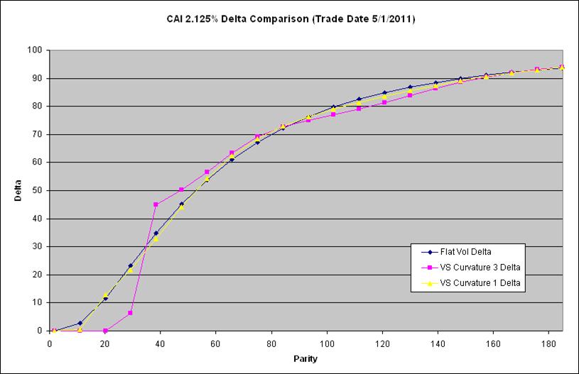
Fig. 13
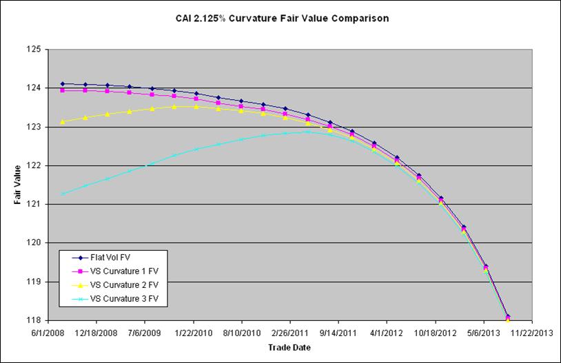
Fig. 14
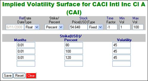
Fig. 15
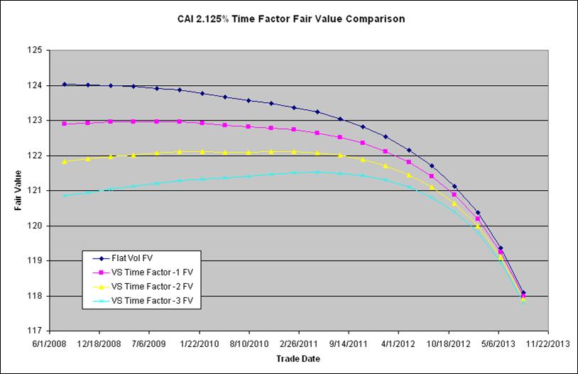
Fig. 16
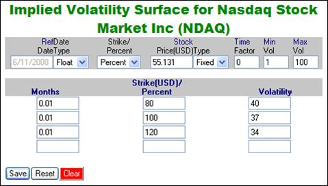
Fig. 17
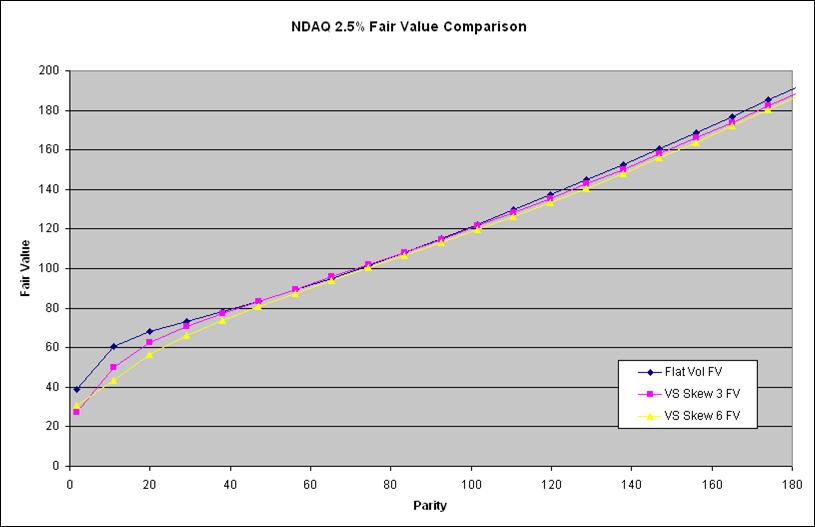
Fig. 18
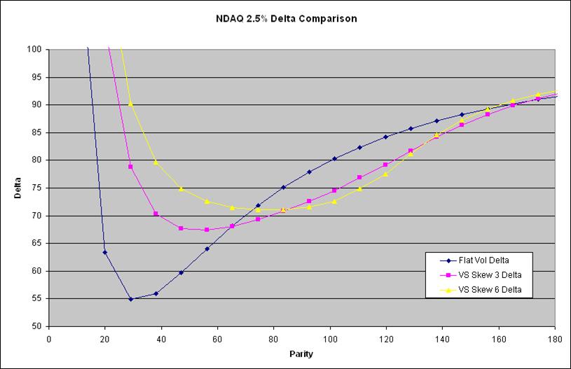
Fig. 19
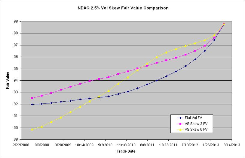
Fig. 20
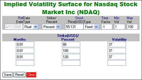
Fig. 21
We now analyze
some other convertible securities. The two most important examples are a
mandatory convertible and a convertible with a variable conversion ratio
(“embedded warrants”). We begin with a mandatory. Up to now, the only way for
you to value a mandatory with different volatility levels was to specify the
low and high strike volatilities in the Value Components section. This is only
an approximation, since a mandatory is really one instrument, not a sum of
separate pieces. For this reason, KYNEX, Inc. does not offer the Value
Components screen for a callable mandatory. A mandatory with 1-1 upside also
cannot be priced using the Value Components screen. However, all of these types
of securities can now be priced using a volatility surface. There is no concept
of a bankruptcy mode for a mandatory, since you receive stock at low stock
prices, and so the volatility surface would in general be a risk-free implied volatility
surface, with (typically) a negative skew. However, there are some important
details because for a mandatory we have a specific concept of low and high
strikes, and the implied volatility levels to input at those strikes.
For our example,
we select the
In Fig. 23 we plot the fair value against the stock price,
using Value Components (blue curve) and the volatility surface (pink curve).
The two valuations are almost equal. Hence the methodology in the Value
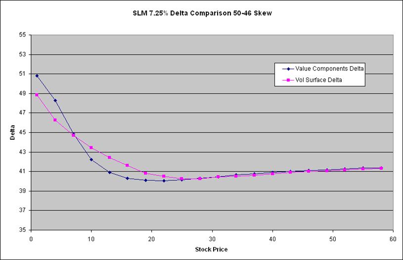
Components screen does give a good approximation for the fair value. The Delta
is however different at parity levels below the high strike. In Fig. 24 we plot the Delta against the stock price. Note that
for a mandatory, we plot the unnormalized
Delta, whereas in all of the previous examples we displayed the Hedge Delta.
The specification of a volatility surface therefore gives a more realistic
estimate of the number of shares to hedge. The Delta obtained with the
specification of a volatility surface is higher (compared to the Delta from the
Value Components methodology) at moderate stock prices, including the zone
between the low and high strikes, and is lower at low or high stock prices.
Fig. 22 Implied Volatility Surface for
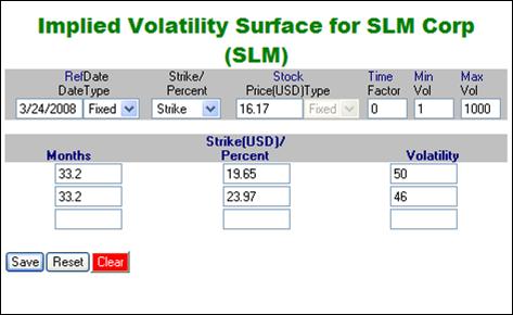
Fig. 23
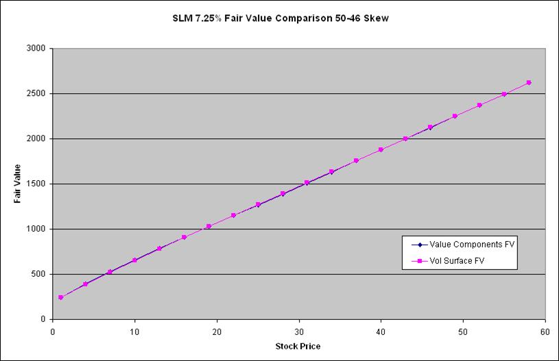
Fig. 24
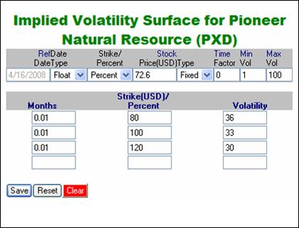
Next, we analyze
convertibles with a variable conversion ratio (“embedded warrants”). Using a
volatility surface allows you to value the contribution of the embedded options
with greater precision. We select as our example Pioneer Natural Resources (
Fig. 25
We plot a graph
of the fair value against parity in Fig. 26. The blue
curve is the fair value with a flat assumed volatility of 41.2%, and the pink
curve is the fair value using the volatility surface displayed in Fig. 25. The valuation using a volatility surface is
slightly lower than the valuation using a flat volatility, as expected. In Fig. 27 we plot the Delta against parity, again using blue
and pink respectively for the valuations using a flat volatility and a
volatility surface. The basic structure of the graphs of the fair value and Delta
are in fact not very different from that of the
Fig. 26
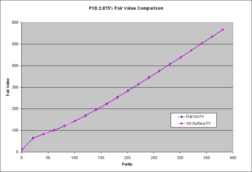
Fig. 27
General Remarks on Specifying a Volatility Surface
Volatility
surfaces can be saved and retrieved from the database. The valuation of a security will remain the same as before, if you do
not specify a volatility surface. Note that a volatility surface is
attached to an underlier, not a
derivative. This has the following consequences:
·
All
convertibles/options on a given underlier will see the same volatility surface.
·
You can choose, on a security-by-security basis, whether
or not to consider the volatility surface. Hence GM A can be valued with a
volatility surface, but GM B can be valued with a flat volatility. However, if both GM A and GM B are valued with a
volatility surface, it will be the same
surface for both.
·
A volatility
surface can also be specified in the New Issue Analytic, to price a
hypothetical new security. However, note that we only allow you to save one volatility surface, although you can
save up to ten scenarios. Hence, when pricing using a volatility surface in the
New Issue Analytic, you must edit and update the volatility surface whenever
you switch from one scenario to another.
In general,
there are two ways for you to create and maintain a volatility surface:
·
You can create a
surface with a fixed date, fixed strikes and a fixed reference stock price.
This is typically what will happen if you create a surface using the implied
volatilities from the listed equity options market, for example. If you create
the surface using listed options data, it will be a surface of risk-free
implied volatilities, and should be used in conjunction with the bankruptcy
mode.
o
The advantage of
this method is that the data will be current with the listed options market.
o
The disadvantage
of this method is that you have to update the surface every day.
o
Another
disadvantage is that, if the surface is not updated every day, the
interpolation of the volatilities, to construct the local volatility surface,
will be based on the surface date (i.e. out of date).
·
You can create a
surface with a floating date and specify the strikes as percentages, with a
floating reference stock price. This could be either a risk-free or a risky
volatility surface.
o
The surface will
maintain its shape and the at-the-money implied volatility will track with the
current spot price. This may be a simpler way to maintain a volatility surface.
The surface does not need to be updated every day.
o
The
interpolation of the volatilities to construct the local volatility surface
will be based on the current trade date. As such, the “months” will reflect the
actual terms to expiration.
o
The disadvantage
of this method is that if the underlier spot price changes significantly, especially
if there is a sudden change to market conditions, then the volatility surface
may not accurately reflect the conditions in the market.
Note also the
following points:
·
If a volatility
surface is blank, then the valuation model will employ the flat (assumed)
volatility.
·
The implied volatility is calculated in the
same way as before. The implied volatility is always defined to be the flat volatility such that the theoretical fair
value equals the Market Price of the security.
·
The implied spread will, however, be
affected by the specification of a volatility surface. The implied spread
calculation will consider the volatility surface when calculating the fair
value.
·
If the valuation
date is in the future, then the valuation model will interpolate forward
volatilities (analogous to the concept of forward interest rates for a yield
curve). The valuation will be based on the forward volatility.
·
The Vega sensitivity is calculated by
applying a parallel shift to the (internally generated) local volatility surface.
In general this is not a parallel shift of the input implied volatilities.
·
For Delta (also Gamma), the sensitivity to a
change in the stock price will in general also include a contribution from the
change in the local volatility.
Since you still
have the ability to input an assumed volatility instead of a volatility
surface, this leads to the following consequences in these situations:
·
Sensitivity
screen
o
If you sweep the
volatility (either dimension 1 or 2), then you cannot specify a volatility surface.
The valuation model will consider the volatility surface instead, and disregard
the volatility sweep.
·
Impact analysis
o
You cannot specify
a volatility surface to price securities for Impact Analysis. A shock to the
volatility will change the value of the flat assumed volatility. The tuner of
RefImpVol will apply to the flat assumed volatility.
·
Options
o
Kynex treats an
assumed volatility of zero to mean that an option should be valued using the
implied volatility. However, if you specify that an option should be valued with
a volatility surface, then that surface will be used even if the assumed
volatility is specified as zero.
o
Hence, an option
will be valued using the implied volatility only if the assumed volatility is
zero and you do not select a volatility surface.
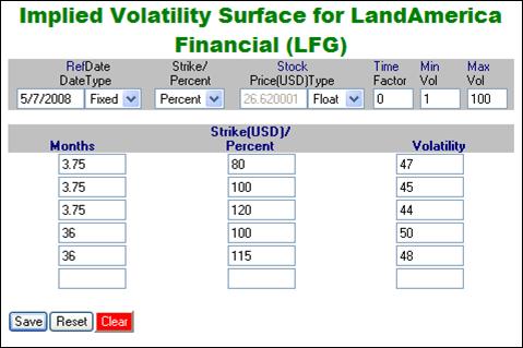
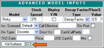
Creating/Editing the Volatility Surface
On the bottom
left corner of the details page (under the Advanced Model Inputs section) you
will now see a button and check box which enables you to value a security using
a volatility surface (see Fig. 28). To create the volatility surface, first click
on the “Vol Surface” button. After
clicking on the button a new window will appear (see Fig. 29).
A similar button will also appear on the valuation page for equity options (see
Fig. 30). Fig. 31 shows a volatility surface using percent strikes (as
opposed to fixed strikes in Fig. 29).
Fig. 28 Convertibles Valuation
Page Showing Button for Volatility Surface
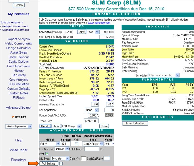
Fig. 29

Fig. 30 Options
Valuation Page Showing Button for Volatility Surface
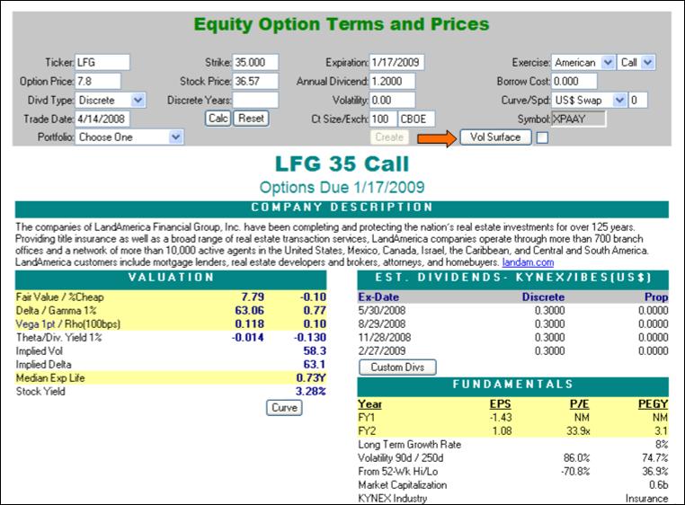
Fig. 31
The
following is a list of definitions which details the inputs for the volatility surface:
RefDate- The
date from which the model interpolates the volatilities. This can be
either a fixed date or a floating date. The type of date is specified in the
drop-down box.
- A
fixed date will assume the implied volatilities are interpolated from the
specified date. You may enter a fixed date that is earlier than
today. Entering a date earlier than
today will produce a warning message that reads “The surface date is earlier
than today, do you want to save with an old date?” If you would like to save the surface
with an old date, simply click OK.
The model does not allow you to enter a future date.
- A
floating date means the interpolations will be calculated from the input
trade date.
Strike/Percent- This
field will specify if the strikes entered in the volatility surface are fixed
numbers or percentages of the reference spot price. Note that when fixed
strikes are input, the values should be expressed in the local currency.
Stock Price & Type- This
field specifies the underlying spot price at which the implied volatilities
were determined. If percent strikes are specified, then they will be a
percentage of this stock price. Values
of less than or equal to zero are not allowed.
A floating reference spot price, and strikes which are
percentages of spot, is useful if you have the view that the volatility surface
will retain its shape for small day-to-day movements in the stock price.
Time Factor- The percentage rate (annualized) at which the volatility surface
will compound or decay beyond the last expiration date specified in the in the
surface. In the example above, the input
of -1 means that the volatilities will decay by 1% every year after 36 months.
Min Vol- The interpolated volatility is not allowed to go below the
minimum volatility value.
Max Vol- The interpolated volatility is not allowed to go above the
maximum volatility value.
Months- The interval (measured in months from the RefDate) to which
the strikes and implied volatilities apply. Decimal values are allowed but
values less than or equal to zero are not allowed. (Example: 1.5 would indicate
1 month and 2 weeks from RefDate). If
you would like to delete an existing row, delete the value you have input in
the months field for the row you want to delete. When you click the save button, the surface
will be saved and the row will be deleted.
Strike/Percent- The strike value of the implied volatility. This can be a
fixed number, or a percentage of the reference spot price, but values cannot be
equal or less than zero.
Volatility- The implied volatility for the given month and strike
inputs. Values cannot be equal or less
than zero.
After entering a surface you should
click the “Save” button. You can also save
a surface by clicking “Enter” at any time.
When the surface is saved, the rows will automatically be
sorted according to the Months, then Strikes (in ascending order).
Reset Button- This
will restore the surface to the last state which was saved in the database.
Clear Button- This will prompt an automatic warning. If you click “OK”
it will blank all the rows and restore all values to their default settings
(e.g. the date). Note that this only
clears the screen, not a surface saved in the database.
Once you are satisfied with the
volatility surface, save it and exit the screen. Then return to the details
page and check the box next to the “Vol Surface” button.
After checking this box, you should then
click the “Recalc” button. The valuation
will now include the volatility surface which you have entered. You may enter one volatility surface per
equity.
Risky and Risk-Free Implied Volatility
The concept of
implied volatility is well-known to market practitioners, especially in the
context of the listed options market. Convertible bonds contain embedded option(s),
hence they also have implied volatility. However, subtleties are involved when
attempting to compare the implied volatility of a convertible to that of listed
options. A convertible is valued on a risky basis; whereas exchange traded
options are valued on a risk-free basis. This leads to the concept of a “risky
implied volatility” for a convertible bond.
Temporarily
ignoring the put and call features of a convertible bond (also the complications
of dividend protection, etc.), a common practice is to visualize a convertible
bond as a risky straight bond plus a risk-free American call option. However,
this viewpoint has the weakness that it assumes the bond floor will hold at low
parity. A better visualization is as follows: at low parity, a convertible bond
behaves as a stock plus a European put option and cash equal to the present
value of the coupon cash flows (the coupons are of course not affected by the
volatility). Note that the above put option is written by the issuer of the stock. As the stock price declines to zero,
the put goes deeper into the money, but
the issuer’s ability to honor the put becomes more and more questionable.
Unlike a listed option, a convertible bond is not guaranteed by an exchange, hence an investor is not guaranteed that the embedded put
will be honored. For this reason, one should value a convertible on a risky
basis (the credit spread indicates the issuer’s creditworthiness). The implied
volatility of a convertible bond is effectively the implied volatility of a risky European put: it is a “risky
implied volatility.” Another way to state this is the implied volatility of a
convertible is the volatility an options broker would be willing to pay for a
put whose ability to collect when it gets in-the-money is tied to the credit
worthiness of the issuer. Note also that the visualization of a convertible as
a straight bond plus call option, or as a stock plus put option, is only
approximate. The option embedded in a convertible does not have a fixed strike
or expiration. The effective strike of the embedded option is a function of the
time to maturity. An approximate measure of the expiration of the embedded
option is the median life of the convertible. Hence when we speak of a “risky
put option” or a “risk-free call option” we are not implying that a rigorous separation of the option from the
convertible bond exists.
On the other
hand, because exchange-traded listed options are guaranteed by the exchange, a
listed put option will be honored even if the underlying stock price goes to
zero. Hence for a listed put option, its implied volatility is “risk-free.” As
such, it is not valid to directly compare the risky implied volatility of a
convertible with the risk-free implied volatilities of exchange-listed options.
Another important point to note is the relationship between observed
volatilities in the stock market and risky/risk-free volatilities especially
during periods of credit crisis. When the observed volatility of a stock
increases in conjunction with stock price decline and credit deterioration, the
risk-free volatility (listed equity options) also increases. However, the risky
volatility decreases as the ability of the issuer to honor the option
diminishes. As a result, convertible securities rarely benefit from the spike
in the risk-free volatilities in such situations. The convertible market has
witnessed this phenomenon time and time again during periods of flight to
quality such as the stock market crash in 1987, the LTCM crisis during 1999,
and the credit crisis during 2007.
We are pleased
to introduce a new metric - “Estimated Risk-Free Implied Volatility” which
gives an equivalent risk-free implied volatility for a convertible bond. Note
that this number is an estimate: it
is calculated by valuing the entire convertible as one security (including all
put and call features, etc.), but the option(s) embedded in a convertible bond
cannot necessarily be expressed as a single (put or call) option with a
definite strike and expiration. The estimated risk-free implied volatility is
an approximate number to back out the credit risk described by the credit
spread specified in the valuation of the convertible. It is calculated using
the risky implied volatility and adjustments based on various internally
computed sensitivities (partial derivatives) to the credit spread, etc. The
estimated risk-free implied volatility is higher than the risky implied
volatility. This is consistent with the fact that investors are willing to pay
a higher implied volatility for a riskless asset than a risky asset. Note that
we do not report this metric for a mandatory or capped convertible, which can
have negative Gamma (or Vega) because they contain embedded short option positions. Furthermore, the
above methodology is based on first-order derivatives. If the credit spread is
large (for example 1000 bps), then the estimated risk-free implied volatility
may come out much higher than the risky implied volatility, but this is not
necessarily a reliable extrapolation.
We only report
the Estimated Risk-Free Implied Volatility when a convertible is valued using
the risky basis (our recommendation), because this methodology values the
entire convertible in a consistent manner. We do not report this metric if the
“Bond+Option” or “Blended” methodologies are specified, where the convertible
is artificially decomposed into pieces valued with different credit spreads.
Note also that if the bankruptcy mode is switched on, then the collapse of the
bond floor at a zero stock price is explicitly included in the convertible bond
valuation. This fact is reflected in the implied volatility. Hence in this case
we also do not report an estimated risk-free implied volatility.
For volatility
surfaces, the input surface is taken to be a set of risky implied volatilities. If you input risk-free implied
volatilities (for example the implied volatilities of exchange-listed options),
then you should also employ the bankruptcy mode, with an appropriately chosen
decay factor that captures the relationship between stock prices and credit
spreads. The bankruptcy mode will capture the risk associated with default by
the issuer, as the stock price goes to zero.