KYNEX Bulletin
October 2009
We are pleased to announce the release of a few enhancements to our convertibles valuation model. Our calculator now supports the use of the stock history in the valuation of convertibles with provisional calls, mandatory convertibles, convertibles with variable conversion ratios (also known as “embedded warrants” or “hyper-structures”), and conversion price reset features.
- For a provisionally callable convertible, the effect of the stock history can be significant if the stock has been trading close to the trigger level, and only a few more days are required to pass the “20 out of 30 trading days” threshold for a provisional call.
- The cases of variable conversion ratios, mandatory convertibles and convertibles with conversion price resets, all share the common feature that the conversion ratio (on the warrant expiration date, or a reset date, etc) is set based on the average stock price over the previous N trading days (where “N” may be 10 or 20, etc.). If the stock history has been trending upwards or downwards significantly, then the average stock price can be significantly different from the current underlying spot price.
We summarize noteworthy aspects about the different types of convertibles below. More details are given in separate sections later in this bulletin.
- Provisional Call
- It is possible that if a provisionally callable bond is not called by the issuer when the threshold is met, the bond may cease to be callable at a later date as the stock prices drop below the threshold. This was in fact the case for the bond HAS 2.5%, due December 1, 2021. The bond was callable in January 2009, up to January 26, 2009, but not from January 27, 2009 into February 2009. An analysis of this bond is given below.
- Depending on the stock price history, the sensitivities of a provisionally callable convertible can be significantly affected. As the stock history approaches meeting the threshold for the call, delta rapidly approaches 100, median life rapidly approaches call notice period, and the fair value approaches parity plus any potential make-whole amounts.
- Mandatory Convertible
- The stock price history is only relevant if the settle date is within twenty days of the maturity of the mandatory.
- The stock price history is used solely to establish the applicable conversion ratio on the maturity date. The actual parity (or terminal fair value) of the bond will depend on the underlying spot price on the maturity date and the computed conversion ratio based on the average stock price.
- If the stock is trading in a narrow range, the average stock price will not be much different from the current spot price on the trade date. However, if the stock price is trending (upwards or downwards), then there could be a significant difference between the average stock price and the current spot price, so the terminal conversion ratio will be significantly different from a value calculated based only on the terminal spot price.
- Variable Conversion Ratio (Embedded Warrants)
- The adjustment to the conversion ratio takes place on the warrant expiration date, and remains in effect for the remainder of the life of the convertible.
- If the convertible is callable, and there is also a put, on the same date as the warrant expiration date, then typically the valuation model will predict that the bond will terminate on that date (either a call by the issuer, or a put or voluntary conversion by the investor). However, there are several issues where the embedded warrants expire on the maturity date on the convertible. An example is LNCR Tranche B 2.75% (due November 1, 2037). Note that this bond has a put on November 1, 2014, which is also the first call date (unconditional call). The valuation model predicts that the bond will terminate on November 1, 2014, and the median life of the bond goes up to this date. However, if for any reason the bond does not terminate on November 1, 2014, then the conversion price calculated on that date will remain in effect until 2037.
- Conversion Price Reset
- The stock price history is only relevant if the settle date is within ten days of the next upcoming reset date.
- If the average stock price is far below the floor price, or far above the current conversion price, then the reset of the conversion price (if any) will be predictable. (Our observation is that this is generally the case.)
- However, if the average stock price is between the floor and the current strike, then the valuation of the convertible will be significantly affected by the stock price average.
The stock history can play a significant role in the valuation of a provisionally callable convertible if the recent stock history has been close to the trigger level, and has exceeded the trigger level for several of the previous 30 trading days. In such a scenario, a call by the issuer may be imminent, and this fact will alter the Delta of the bond (and therefore influence stock hedging decisions). We made a synthetic convertible bond with a provisional call feature. The trigger stock price is 17.58 and the issuer can call only if the stock price has been at or above the trigger level for at least 20 out of the last 30 trading days. We valued the bond on successive trade dates, from 9/3/2009 through 10/12/2009. We created a simulated stock history as follows.
- The stock price was below 17.58 for dates on or before 9/10/2009.
- On the dates 9/11/2009 and later, the stock price was 18.58, i.e. $1 above the trigger level.
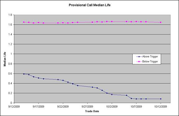
Hence, on each successive trade date starting from 9/13/2009, the stock history was above the trigger for an additional day. On 10/7/2009, the stock history was above the trigger level for 20 days, and the issuer was able to call the bond. We display the valuation of the bond in Fig. 1. The blue curve in Fig. 1 shows the fair value vs. trade date (the pink curve is for a different simulated stock history, and will be discussed below). As expected, the fair value (blue curve) declines because of the imminent approaching call by the issuer. The fair value bottoms out once the issuer is able to call the bond. In Fig. 2, we display a graph of Delta (blue curve) for the same set of trade dates. We see that Delta increases and reaches 100 on 10/7/2009, i.e. when the issuer is able to call the bond. In Fig. 3, we display a graph of the median life (blue curve) for the same set of trade dates. The median life decreases, reaching 30 days (i.e. the call notice period) when the issuer is able to call the bond.
Next we created a simulated stock history, for the same bond, but where the stock price was always 16.58, i.e. $1 below the trigger level. In this case the issuer was not able to call the bond on any of the trade dates in our analysis. In Fig. 1, the pink curve shows the fair value on the successive trade dates. We observe that the fair value (pink curve) does not change much on successive trade dates. In Fig. 2 (Delta, pink curve), we observe that the Delta of the bond also does not change much on successive trade dates. (It is always slightly below 50%.) Hence the Delta can differ by as much as 30-50 points relative to the previous scenario. In Fig. 3 (median life, pink curve), we observe that the median life does not change much with time, and is always slightly greater than 1.6 years. This value is much higher than the blue curve (where the issuer can call the bond), where the median life is 0.6 years or less.
It is of course possible to create scenarios with many other possible simulated stock histories. The above cases are only two extreme examples. We see that, depending on the stock history, the behavior of Delta can be significantly different. In one case Delta does not change much with time, whereas in the other case it varies significantly and eventually reaches 100. The difference in the behavior of the median life (blue and pink curves in Fig. 3) also reflects the influence of the stock history.
Fig. 1 Provisional Call Fair Value
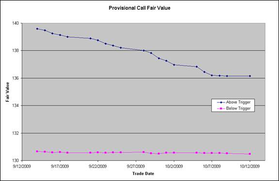
Fig. 2 Provisional Call Delta
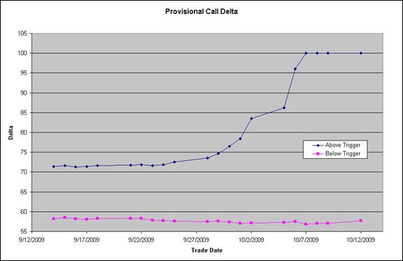
Fig. 3 Provisional Call Median Life
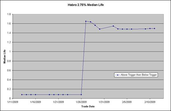
To illustrate the basic issues in more detail, we searched for historical data for convertibles with provisional calls, to find examples of bonds where the history of the underlying stock was close to the trigger level. One such example is Hasbro 2.75% due December 2021, for trade dates in January 2009. The stock history of Hasbro in December 2008 and January 2009 was such that the bond was callable in January 2009, for trade dates up to and including 1/26/2009. However, on 1/27/2009 the bond was not callable because on that date, the stock history was above the trigger level for only 19 out of 30 days. The bond was also not callable on the subsequent trade dates in Feb 2009. Fig. 4 shows a time scan, where we plot the fair value against the trade date from 1/13/2009 through 2/11/2009. We see that the fair value takes a step up from 1/26/2009 to 1/27/2009, because the issuer was not able to call the bond on 1/27/2009 onwards. In Fig. 5 we plot the median life, for the same date range. We see that the median life also takes a step up, from about 0.1 years to about 1.1 years, an increase of about 1 year.
Fig. 4 HASBRO 2.75% Fair Value
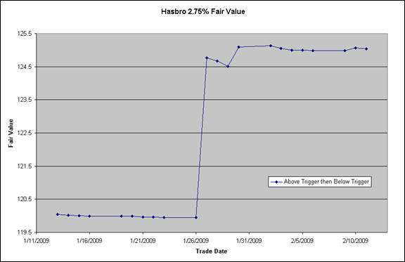
Fig. 5 HASBRO 2.75% Median Life
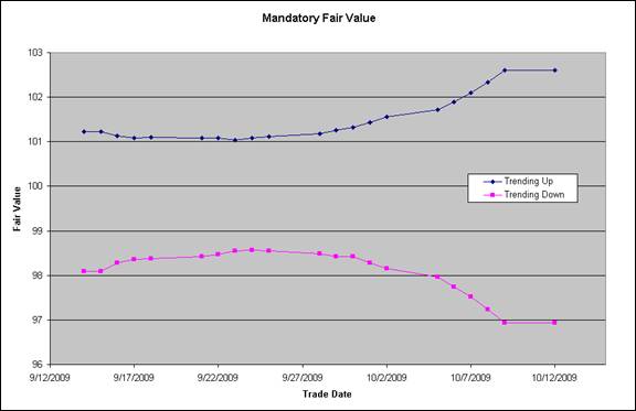
For a mandatory, the conversion ratio is determined using the average stock price for the preceding 20 days prior to the maturity date. We made a synthetic mandatory convertible. The low strike is 61.25 and the high strike is 73.5. We valued the bond under two scenarios:
- The stock price history was trending upwards, such that the spot price on the maturity date was above the high strike, but the average stock price was between the low and high strikes. In this scenario, the terminal conversion ratio would be higher than the minimum ratio.
- The stock price history was trending downwards, such that the spot price on the maturity date was below the high strike, but the average stock price was between the low and high strikes. In this scenario, the terminal conversion ratio would be lower than the maximum ratio.
We valued the bond in a time scan for trade dates from 9/13/2009 through 10/12/2009.
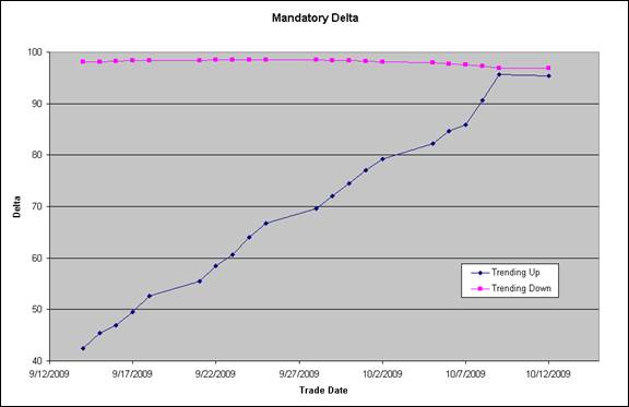
(The maturity date was 10/15/2009.) Fig. 6 shows the fair value on the various trade dates. The blue curve shows the valuation for an upward trending stock price history, and the pink curve shows the valuation for a downward trending stock price history. The fair value in the blue curve initially falls and then increases. This is due to two competing effects. The increase in the spot price on successive trade dates increases the value of the embedded warrants, but the decrease in the time to expiration decreases the time value of the optionality of the mandatory. The overall effect is to produce a graph where the declining time value initially pulls the fair value down, but the increase in the spot price eventually pulls the fair value up. The stock history also contributes to an increase of the fair value, due to the increased conversion ratio. The fair value in the pink curve initially rises and then decreases. This is because a mandatory has negative gamma and negative theta near the low strike, so a decrease in the time to maturity leads to an increase of the time value. This pulls up the fair value. Eventually the decrease of the spot price because of the downward trending reduces the fair value. The stock history contributes in this case to a decrease of the fair value, due to the reduced conversion ratio. In Fig. 7 we plot the Delta on the various trade dates. In both scenarios (blue – stock trending up, pink – stock trending down) the Delta increases steadily towards the respective terminal value. In both cases, this essentially reflects the effect of the declining time to maturity of the mandatory – the Delta approaches the “hockey stick” terminal payoff. The terminal values of the Delta in the two scenarios are determined by the respective stock price histories.
Variable Conversion Ratio (embedded warrants/hyper-structure)
If the embedded warrants in a convertible with variable conversion ratio expire prior to the maturity date, the value of the conversion ratio is reset on the warrant expiration date, using the average stock price for the preceding 20 days prior to the warrant expiration date. The resulting conversion ratio then remains in effect until maturity. This calculation is similar in concept (but different in details) from a conversion price reset. If the stock price history is trending, either upwards or downwards, then the average stock price may differ significantly from the current stock price on the warrant expiration date.
We made a synthetic convertible bond with a variable conversion ratio. The base conversion price is 51.271. We valued the bond under two scenarios:
- The stock price history was trending upwards, such that the spot price on the warrant expiration date was above the conversion price, but the average stock price was below 51.271. In this scenario, there would be no change to the conversion ratio on the warrant expiration date.
- The stock price history was trending downwards, such that the spot price on the warrant expiration date was below the conversion price, but the average stock price was above 51.271. In this scenario, there would be an increase to the conversion ratio on the warrant expiration date, even though the spot price on the warrant expiration date was below the conversion price.
We valued the bond in a time scan for trade dates from 9/13/2009 through 10/12/2009.
(The warrant expiration date was 10/15/2009.) Figs. 8 and Fig. 9 show the fair value on the various trade dates. The graph in Fig. 8 shows the valuation for an upward trending stock price history, and the curve in Fig. 9 shows the valuation for a downward trending stock price history. The fair value in Fig. 8 initially rises and then decreases. This is due to two competing effects. The increase in the spot price on successive trade dates increases the value of the embedded warrants, but the decrease in the time to expiration decreases the time value of the option of the embedded warrants. These two effects work in opposite directions, leading to a graph with a peak in the fair value. Since the stock history is trending upwards, on any given trade date the average stock price is less than the current spot price. This decreases the value of the embedded warrants, also helping to pull down the overall fair value. In Fig. 9, the stock price is trending downwards and the time value is also decreasing. Therefore the curve consistently slopes downwards. The stock history causes the conversion ratio to be increased on the warrant expiration date, but this has relatively little effect on the valuation in this scenario.
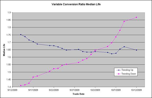
In Fig. 10 we plot the Delta on the various trade dates, for the two scenarios (blue – stock trending up, pink – stock trending down). The Delta declines steadily in both scenarios, indicating the convergence of the Delta to essentially the same value on the warrant expiration date. In Fig. 11 we plot the median life on the various trade dates, for the two scenarios (blue – stock trending up, pink – stock trending down). In the case where the stock price trends upwards, the median life does not change much (approximately 1.7 years), because the valuation model indicates not much change to the parameters of the bond. In the case where the stock price trends downwards, the median life increases steadily (from 1.4 to 1.9 years) as the trade date advances, because the declining value of the optionality of the embedded warrants indicates that there is less incentive to convert the bonds early (or for the issuer to call the bond).
Fig. 8 Variable Conversion Ratio Fair Value
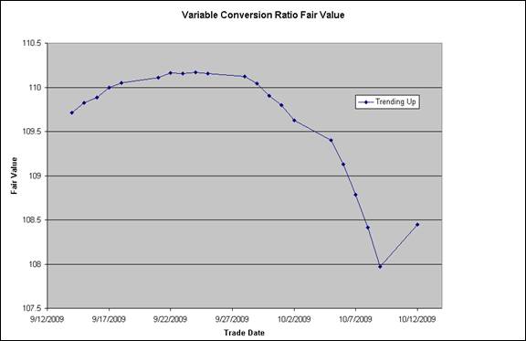
Fig. 9 Variable Conversion Ratio Fair Value
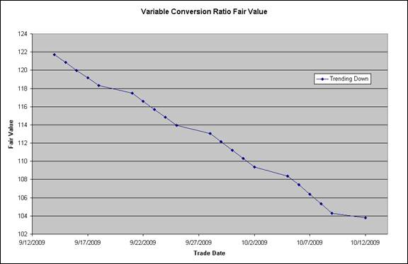
Fig. 10 Variable Conversion Ratio Delta
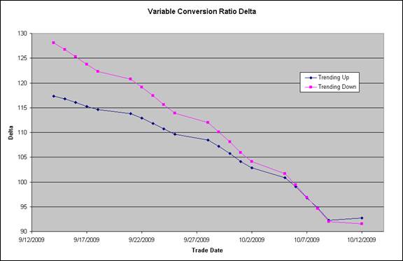
Fig. 11 Variable Conversion Ratio Median Life
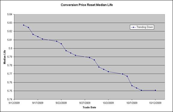
For a convertible with a conversion price reset feature, the conversion ratio is determined using the average stock price for the preceding 10 days prior to the next reset date. We made a synthetic convertible with a conversion price reset. The initial conversion price $9.292 with a floor of 80% (= $7.4336). We valued the convertible using a downward trending stock history, such that the spot price on the maturity date was below the floor value, but the average stock price was between the floor and initial conversion price.
We valued the convertible in a time scan for trade dates from 9/13/2009 through 10/12/2009. (The reset date was 10/15/2009.) Fig. 12 shows the fair value on the various trade dates. The fair value decreases monotonically as the trade date increases. This is because of the decline in the stock price. The effect of the stock price history is to accentuate this decrease, because the conversion ratio does not increase to the maximum value (because the average stock price is higher than the floor value of 7.4336). In Fig. 13 we plot the Delta on the various trade dates. The value of Delta increases steadily, reflecting the influence of the imminent increase to the conversion ratio. The value of Delta on the reset date is obviously determined by the average stock price calculated from the simulated history. Fig. 14 shows a plot of the median life on the various trade dates. The value of the median life decreases steadily, from 5.83 to 5.75 years, which is simply the decrease in the time to maturity of the bond, by the 30 days of the time scan. Hence in this scenario the median life is simply the time to maturity, and does not depend on the stock history.
Fig. 12 Conversion Price Reset Fair Value
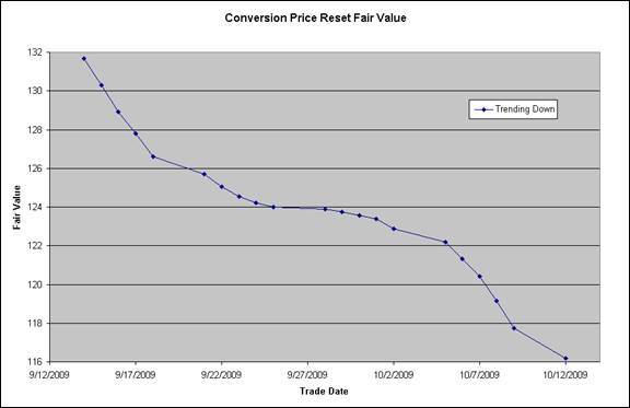
Fig. 13 Conversion Price Reset Delta
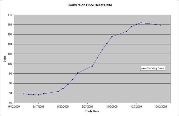
Fig. 14 Conversion Price Reset Median Life