KYNEX Bulletin
December 2006
CDS
Valuation & Recovery Rate Model
The Kynex Credit Default Swap (CDS) Model (as described in the June 2004 Kynex Bulletin) has been enhanced significantly. Model changes and their benefits are highlighted here, and you can follow the links for additional detail and explanation.
v
The Kynex CDS calculator now accepts a credit curve (term structure of CDS spreads). In the very near future, you will be able to
store the credit curve for a specific credit and maintain offsets for debt
subordination level, and contract specific items such as documentation type,
settlement type, and recovery type. Therefore,
you can consistently mark multiple CDS contracts on a credit from a single term
structure. You no longer need to mark
every individual CDS. You no longer need
to get quotes on contracts whose remaining life to maturity does not match any
tenors for which quotes are readily available in the market. If the term structure on a given credit
remains unchanged, you no longer need to mark these contracts, we will be able
to re-calculate the unwind value. As the
contracts age, mark-to-market will remain accurate. You
will spend less time gathering and marking CDS instruments and more time
identifying and managing your investments. For details on providing the
credit curve inputs to our calculator, please see the description of our valuation screen.
You will be able to maintain your
credit curves through the Credit Curve Maintenance Screen (and/or by ftp from a
third party provider).
v
The calculator now accommodates the market
convention of quoting to the next IMM roll date as
well as on a constant maturity basis. If a tenor type of IMM roll is chosen,
the calculator also quantifies your P&L on the next roll date as well as
the drop in CDS spread assuming the broker does not remark the CDS on the roll.
v The Kynex CDS calculator now offers an optional recovery rate model which simulates the expected relationship between CDS spreads and recovery rates. The model will also calculate the implied flat recovery rate while leaving default rates unchanged. The model can help identify potential pricing errors in the market based upon your expectations of realizable recovery rates upon default. This model is intended to address the “downturn LGD” (loss-given-default) concerns in the Basel II framework document (paragraph 468). The negative correlation between default rates and recovery rates will amplify the effects of economic cycles, and this expected behavior should not be overlooked from a risk perspective.
v The Kynex CDS calculator now offers equity-linked delta and gamma estimates. These measures help estimate the impact of stock prices on the value of a CDS. They will help you with the difficult task of hedging portfolios consisting of equity derivatives (e.g. convertibles and options) and credit default swaps. Please refer to our equity-linked portfolio hedging example.
v CDSs on distressed credits are now frequently quoted in terms of a running spread plus upfront points. The Kynex CDS calculator allows for such market quotes, thus saving time analyzing such contracts (an equivalent flat spread is calculated).
v The economics of hedging credit spread risk with CDSs is discussed. A fixed income portfolio hedging example shows four alternatives. The profit and loss on equity-linked portfolios using CDS and a long convertible position as well as a short stock position is also examined.
Hedging Fixed Income Portfolios with CDS
We analyze a 5-year bullet
corporate bond hedged with CDS of varying maturity. Our findings are as
follows:
·
If protection against a default event is the
major consideration, it is economical to hedge with the shortest duration CDS
to cover the expected default at the risk of spread DV01 mismatch and
inadequate protection against credit deterioration.
·
If protection against credit deterioration is the
major consideration, it is economical to hedge with a liquid CDS longer than
the maturity of the corporate bond at the risk of spread DV01 mismatch and
inadequate protection against a default event.
·
You could achieve protection against both a
default event and credit deterioration via a hedge made up of a short duration CDS
and a long duration CDS without sacrificing spread DV01 match at the risk of
managing a complex hedge.
When faced with hedging credit
spread risk on a fixed income bond with a CDS contract, most market
participants would not buy a CDS whose triggering credit event is a credit
downgrade. This approach would be expensive, and partial downgrades would be
ignored. Rather, you would buy long protection on a corresponding single name
CDS. This discussion assumes the
portfolio to be hedged consists of a long position of $5 million GMAC corporate
(the techniques evaluated here could also apply to a whole portfolio of bonds
and DJCDXs as the hedge). On 8/1/2006, we assumed a
GMAC term structure of 154.25bps for the
one year, 191.6 bps for the three year, and 224.8bps for the five year (longer
contracts were not quoted). Our terminal horizon date is assumed to be
The table below (details are in the Appendix) shows four approaches you might use. In all cases, the notional amount of the CDS is determined by matching the spread DV01 of the CDS with that of the corporate bond.
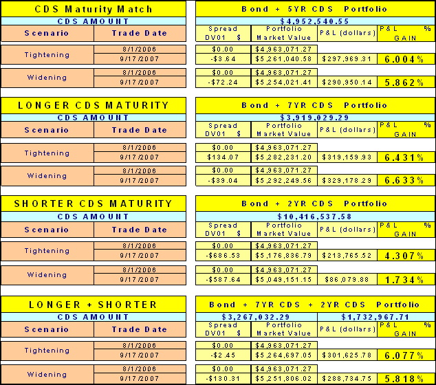
The standard way to hedge is to buy long protection on a CDS that
closely matches the remaining term of the corporate bond. In our example, you
need to buy about $4.95 million of a five year CDS. The spread DV01 tracks well a year from now
under both a tightening and widening scenario.
In the event of default however, the CDS does not quite cover the bond
(you would have needed to buy a full $5 million). If the DV01 of the bond is
significantly smaller than that of the CDS, this small difference in this
example can grow. The economics of hedging
with a longer duration CDS appears attractive if you are relatively
unconcerned about default. Under this
scenario, you take advantage of the lower notional amount. If you are only concerned with default, then
buying $5 million of the shorter duration
CDS is the way to go. Otherwise, the
shorter duration CDS approach should be abandoned. Buying both a longer duration CDS and a shorter duration CDS so that
notional amounts and DV01s are simultaneously matched appears attractive,
albeit with an additional inconvenience and expense of maintaining two CDS
contracts. This approach might be more
appropriately used on a portfolio of bonds where the CDSs used to hedge are DJCDXs. Even for
a single bond position with an odd remaining term to maturity, a longer duration
CDS with a standard tenor plus a shorter duration CDS with a standard tenor
might be cheaper due to liquidity.
Hedging Equity-Linked Portfolios with CDS
We analyze the Eastman Kodak
3.375% convertible bonds due 2033 hedged with various combinations of stock and
CDS, and our findings are as follows:
·
While it is possible to hedge a long convertible
position via CDS, unless there is a bankruptcy event, the drag on the carry
from the CDS deal payments makes the hedge more expensive than a simple short
stock hedge due to the rebate you collect from the short stock position.
·
Writing a CDS contract as a hedge against a
short convertible position instead of a long stock position would be attractive
if the stock pays no dividend and the coupon on the convertible is relatively
high, since the deal payments from the CDS offset the coupon payments on the
convertible helping the cost of carrying the position.
·
You can also hedge a long convertible position
with a CDS instead of a short corporate bond position if a corporate bond
exists from the same issuer. While the ease of wind-and-unwind as well as not
needing to borrow the short corporate bond make the CDS hedge more attractive,
it is important to realize that the CDS hedge does not provide a meaningful
interest rate hedge while a short corporate bond will.
A short stock position, or a
short call option on the stock, or a long put option on the stock or a
combination of the above are common hedges for a long position in a convertible
bond. Since several convertible securities exhibit an inverse relationship
between the stock price and credit spread (commonly referred to as bond floor
does not hold as the stock collapses) a CDS contract offers another alternative
to hedging. We compute the notional amount of CDS to hedge in two different
ways.
In the first method, we calculate
the difference in theoretical delta assuming the credit spread is independent
of the stock price and assuming a relationship (decay
factor) between the stock price and credit spread. This difference is
hedged via CDS, and the notional amount of the CDS is computed using the decay factor
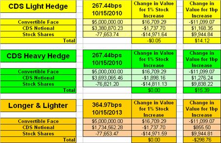
(above) and spread dv01of the CDS. (in our example, the CDS Light Hedge in
yellow).
In the second method, we
calculate the CDS notional based on the spread dv01 of the CDS and the spread
dv01 of the convertible (in our example, the CDS Heavy Hedge in green) assuming
an inverse relationship between stock prices and credit spreads (decay factor). Our CDS calculator computes the
equity delta for the CDS which can be used to compute the effective share
equivalent. The difference between the effective share equivalent and the
theoretical delta of the convertible assuming an inverse relationship between
stock prices and credit spreads in shares would have to be hedged by selling
stock short.
The details for both of these
methods can be found in the Appendix.
Successfully managing credit
spread risk in an equity-linked portfolio starts with some science but
ultimately requires art (and probably some luck as well). We will start by
assuming that our portfolio consists of a $5 million long position of the
Eastman Kodak (EK) convertible maturing
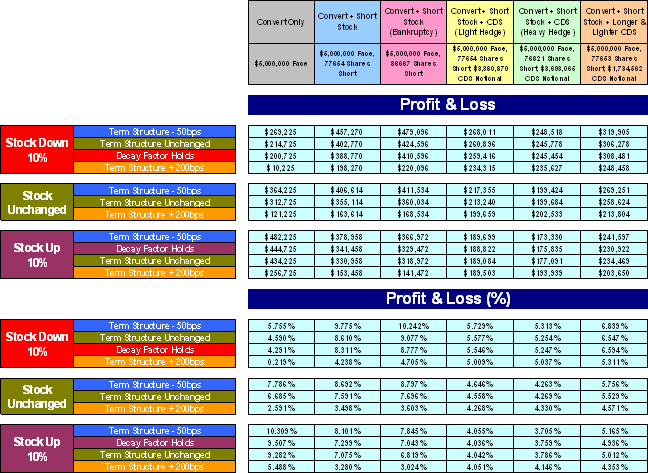
For comparison, we included a
portfolio which is only long the convert, and two portfolios whose equity
exposure is hedged with and without the Convertible Model’s bankruptcy mode. The other three portfolios contain a short
stock position and a long CDS position (please see the Appendix for how these portfolios were
constructed). Not surprisingly, the CDS deal payments really drag down
performance (especially when the rebate rate is high). The “Heavy-CDS Hedge”
portfolio will perform the best if spreads widen dramatically, but the spread
dv01 coverage is expensive. The “Light-CDS Hedge” portfolio demonstrates the
usual way of hedging an equity–linked portfolio, but its performance is still
weighted down by the CDS deal payments. This situation can be partially ameliorated by going longer and lighter on
the CDS. The 7 year CDS has a larger delta and spread dv01. This means you can buy less of the CDS, and
therefore reduce your dollars of deal payments.
Although the coverage is not as good, the “Longer and Lighter CDS Hedge”
portfolio starts at an immediate annualized advantage of $27,112. The advantage
holds until spreads widen out to 277.1 bps or beyond. If you believe spreads will not widen beyond
this, there is no reason to make the additional deal payments. You can adjust your coverage based upon
your assumption on how wide spreads are likely to widen.
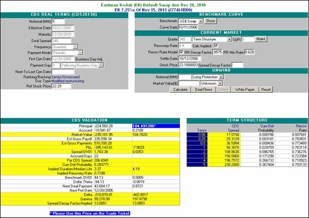
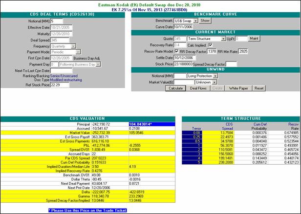
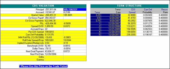
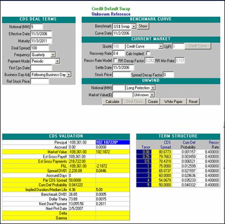
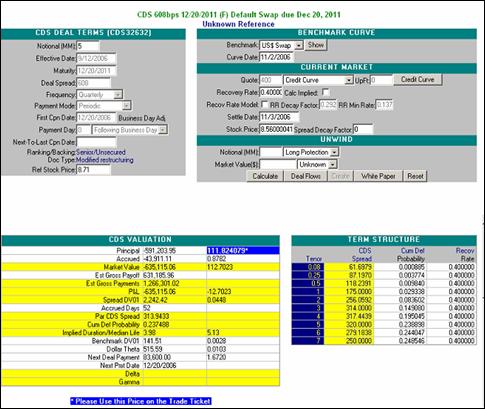
CDS Valuation Screen Description
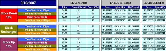
The CDS Valuation Screen (i.e. the CDS detail page) is now composed of several sections. As an example, the following input and output sections use a CDS on an Eastman Kodak straight bond.
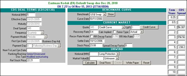
In this example, we show the screens you will see displayed
if you choose the Credit Curve option in the quote type box. A separate section allows you to enter the
desired credit curve. The quote type options are as follows.
CDS Spread
Short Bond Price
Upfront Points
Paid
Upfront Points
Received
Running Spread +
Upfront Points
Credit Curve
If the Credit Curve option is selected, the calculator will
always use the CDS term structure displayed.
If a credit curve has been stored (either from the Credit Curve
Maintenance screen or from an uploaded file), then the Credit Curve Option will
be used at the initialization of valuation.
Additional documentation on
Credit Curve Maintenance will be forthcoming. If you are interested in the
calculation of delta and gamma, you must enter a spread
decay factor. If you wish to use the
Recovery Rate Model, you need to check the Recovery
Rate Model box and override the model
parameters if desired. If the spreads
in the credit curve are IMM roll spreads, then you
should select the IMM roll tenor type. The valuation output section follows.
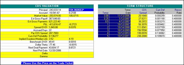
Under the CDS Valuation section, standard values in dollars
and short bond points are shown. The
P&L values assume no unwinds from the effective date until settlement. The
Spread DV01 values show the change in market value for a one basis point
parallel upward shift in the entire credit curve. Similarly, the Benchmark DV01
shows the change in market value for a one basis point upward shift in the
entire benchmark curve. The Par CDS Spread corresponds to the exact maturity
date of the CDS, and results in the identical market value if used as a flat
CDS quote. Dollar Theta shows the change in principal if the settlement is
incremented by one (calendar) day. Delta values show the change in principal
for a 1% change in stock price using the specified spread decay factor for
every point on the credit curve (e.g. the expected short bond price for a 1%
change in stock price equals 104.860243*(1 + 0.01*4.0751) = 109.1334). Gamma values show changes in Delta values
(strictly speaking, the signs of the short bond point values should be reversed
for all of the Greeks as well as SpreadDV01 and Benchmark DV01). If the Recovery Rate Model is turned on, an
implied flat recovery rate can also be calculated. The implied flat recovery rate is computational intensive and time consuming
if a credit curve is specified. If
you choose to calculate it, its value will result in the identical market value
if you then turn off the Recovery Rate Model and specify the flat recovery rate
as that value. The Term Structure
section shows the Credit Curve for additional tenor points. These values (along with additional internal,
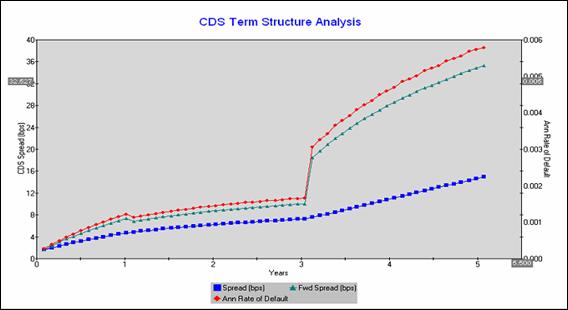
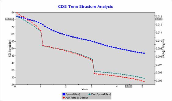
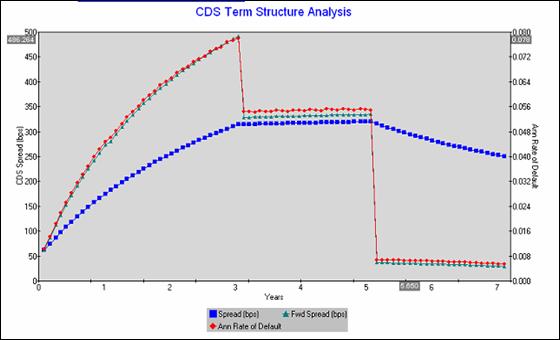
valuation points) are graphed as follows.
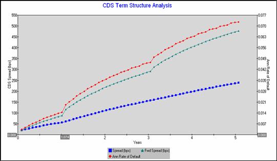
The CDS spreads (blue) and the forward CDS (green) spreads
are plotted versus the left hand axis, and annualized default rates (ADR) are
plotted versus the right hand axis. Forward CDS spreads are the basis point equivalent
of ADRs.
In constructing your CDS credit curves, clients should be careful when mixing CDS
quotes from different trade days or contributors. You can easily wind up with a term structure
fruit salad (apples and oranges).
Consider the ask side CDS spreads shown by Bloomberg™ for IBM on
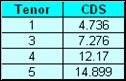
Bloomberg™
clearly marks the 4 year value as originating on
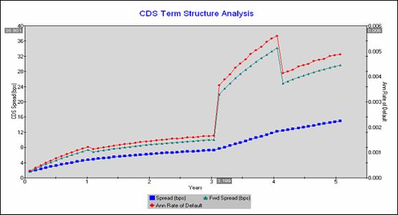
If the 4 year tenor is removed, the analysis shows the
following.
More tenor points will not necessarily make
your valuation more accurate.
If you interpret
the credit curve spreads as IMM roll spreads, then the output section is as
follows. The output tenors are reinterpreted,
and the tenor dates show the future roll dates corresponding to the tenor
points.
The next IMM
roll date is shown as well as the expected P&L drop on the roll date. We
also show the drop in the CDS spread due to the roll.
As noted in the CDS Valuation Screen Description, you can
now enter CDS spreads that conform to the IMM quarterly roll convention. If the “IMM Roll” tenor type is selected,
both input and output CDS spreads will be consistent with this convention. This
roll convention combines the usual daily drops throughout the quarter together at
the beginning of the current roll period.
To see the roll in action, we selected a Kodak CDS as an example and
calculated CDS spreads and unwind values from a constant credit curve for every
trade date over a full quarter starting from 6/20/2006 until 9/20/2006.assuming
both actual and roll tenor types.
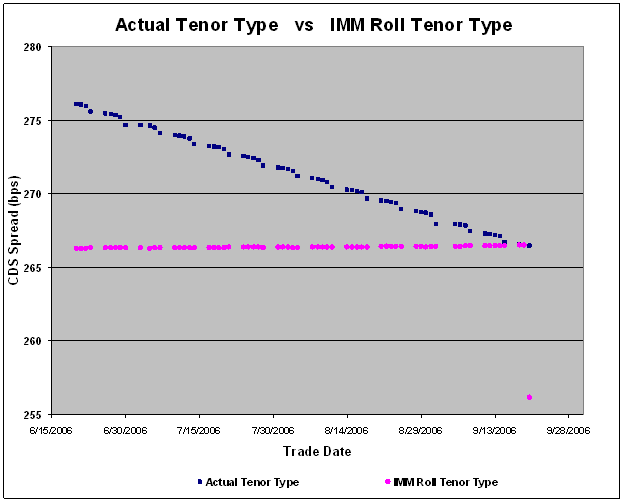
As
expected, the CDS spreads using the actual tenor type exhibits a classic roll-down-the-curve
behavior.
The roll tenor type shows that the CDS spread is flat within the quarterly
period with an abrupt drop when the trade date is on the 20th. On
the 19th, the CDS spreads are identical.
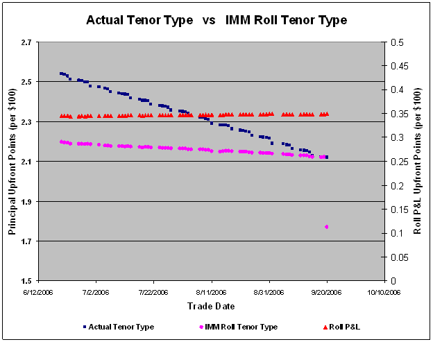
Unwind
values (as measured in principal upfront bond points) also exhibit the same
behavior.
The
Roll P&L value gives today’s expectation of what the drop in unwind will be
on the next roll date. Since the credit
curve was held constant during the quarterly period, the Roll P&L is flat.
If you are long CDS, you should consider
unwinding near the end of the IMM quarter if possible.
Inverted Credit Curves
For most credit curves, the Kynex assumption that CDS
spreads tend toward zero as the time to expiration goes to zero is reasonable.
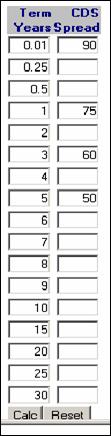
But clients can control their “time 0” values by inserting a tenor at 0.01
years. For inverted credit curves, this
is especially useful. The five year generic CDS shown below illustrates how to
do this.
Impossible Credit Curves
Suppose you believe Ford (F) will begin to improve after
about five years, and will substantially improve by year seven. You might
reflect that on a Ford CDS as follows.
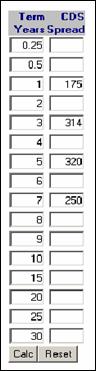
However, if you decided the spread corresponding to the seven year should really be 225, you would get the following.
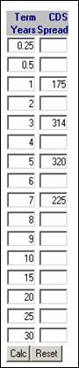
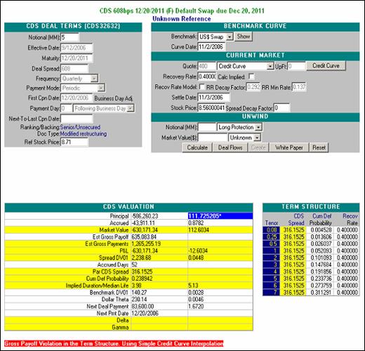
In this case, a flat seven year CDS spread of 225 produces a gross payoff far too low. It cannot be reached from the five year point unless probabilities of default become negative between five and seven years. But this is not possible. In this case Kynex does a simple interpolation on the credit curve to determine a flat CDS, and a flat CDS valuation is performed.
The Kynex Recovery Rate Model arose out of our concerns over risk. The theoretical basis of our model is the work by Altman, Brady, Resti and Sironi in their March 2003 paper entitled “The Link between Default and Recovery Rates: Theory, Empirical Evidence and Implications”.
In that paper, the negative
correlation of default and recovery is effectively explained and
demonstrated. This inverse relationship
has two main reinforcing determinants which act in addition to a default payoff
as merely arising from the residual value of a company’s assets. At the company level, the same economic
conditions that increase the rate of default will also increase default severity. At the market level, higher default rates
means a larger supply of distressed securities. With a larger supply available,
the vulture funds will pay less for the debt of the same distressed
company. The result is a “perfect storm”
scenario in which the “rate of default is a massive indicator of the likely
average recovery rate amongst corporate bonds.”
In order to value a CDS, market participants are faced with an
impossibly difficult task of assigning a recovery rate to a company’s credit
which may be currently rated as AAA. No one knows beforehand exactly how a
company will fare in bankruptcy court, especially one whose credit is so far
away from default. Kynex does not pretend to shed any light on that
question. However the Kynex Recovery
Rate model can provide recovery rates which are consistent, on average, with
specified market CDS spreads. Once a CDS
term structure is given with the recovery rate model turned on, default and
recovery rates are calculated. Recovery
rates can be calculated which are consistent with the 1982-2001 data as
presented in Table 1 (Default Losses, Recovery Rates and Losses) of the paper
mentioned above, or they can be calculated from user specified input for the
recovery rate decay factor and the recovery rate minimum rate. Please refer
to the recovery rate section of the
Appendix for a description of the Kynex methodology. You must decide if it
is more realistic to use a flat recovery rate or a recovery rate that adjusts
for rates of default.
Although
you must create and store individual single name CDSs, DJCDX issues are already
stored in Kynex for your use. As new
issues come out, their contract terms will be entered into Kynex by our staff. You
can access them by the Bloomberg™ deal number
(e.g. the CDX.NA.IG.6
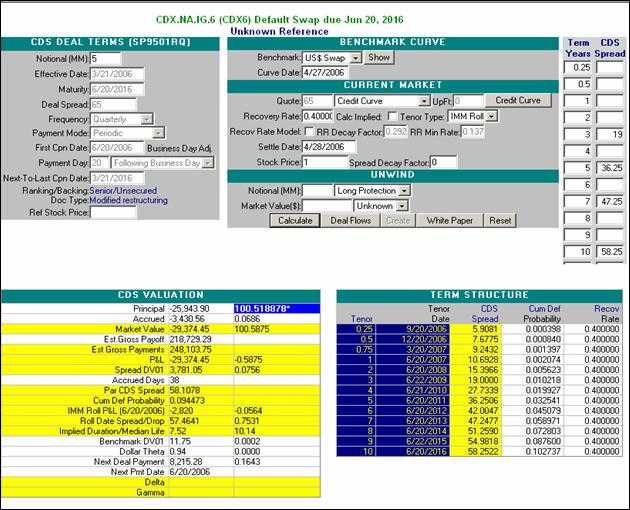
The term structure will price the
underlying quoted contracts accurately. Any variation is due to business day
adjustments and to a different cycle (the CDX contracts cycle on the 20th,
while the underlying calculation uses a cycle based upon the settlement date,
e.g. the 28th in this case).
Even though the earliest quote is on the 3 year contract, Kynex will
price the shorter contracts as well. This extrapolation is based on model
defaults and the Kynex belief that CDS spreads tend towards zero on settlement.
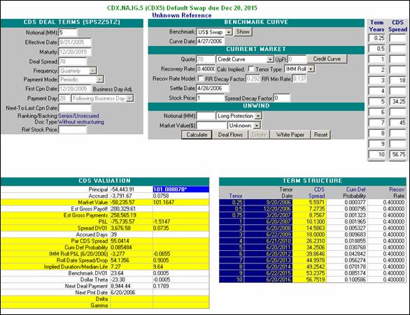
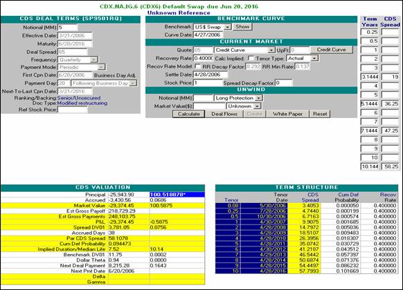
If you want to compare the CDX5’s to the CDX6’s, an additional valuation is
required.
If you desire constant maturity spreads (e.g. credit
spreads), then you need to switch to the actual tenor type, and compute
fractional tenors for the spreads.
Kynex CDS Model Appendix
Hedging Fixed Income with CDSs (Detail
Table)

Valuation Model Comparisons
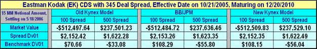
Although the Kynex model has undergone substantial changes, your current valuations and risk measures should be relatively unchanged. As an example, we show valuations on an Eastman Kodak CDS assuming flat market spreads of 100 and 500 and a flat recovery rate of 40%.. The columns labeled “BB/JPM” show values based upon the Bloomberg™ JPM CDS model. The new Kynex model will give benchmark DV01 values more in line with the JPM model (Kynex changed the definition slightly).
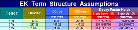
Historical Spread Decay Factor
For the EK 3.375% 10/15/2033 (10/15/2010) convertible bond., the graph below plots daily stock prices starting on 4/3/2006 and through 8/10/2006 versus three year and five year mid-level CDS spreads over the same interval. These values are readily available on Bloomberg™, for example.
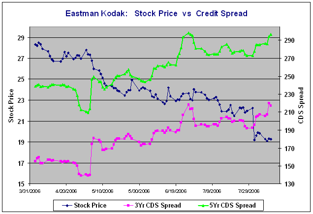
This graph
depicts an almost classic inverse relationship between stock prices and credit
spreads. EK posted a widening first-quarter loss on

A positive decay factor indicates an inverse relationship
between stock prices and spreads. This data can be used in at least three ways
to get an estimate of the spread decay factor. The results of the three methods
are summarized below.
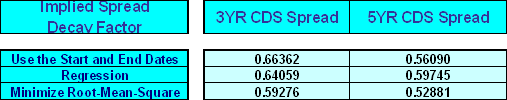
Stock prices and spreads at the starting and ending points can be used. You can also get an estimate of the decay factor by using the following regression formula.

Alternatively, you can determine the decay factor that minimizes the following equation.

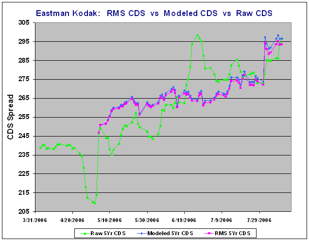
The following graph shows how the modeled spreads track the actual raw spreads for the five year CDS.
As can be seen by the difference between the 3 year and the 5 year decay factors, decay factors have a term structure.
Hedging Equity-Linked
Portfolios with CDSs (Details)
On
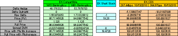
Calculating the CDS Notional Given a
Desired Equity Hedge
![]()
![]()
![]()

Calculating the CDS Notional from Spread
DV01
![]()
The implied
volatility on the convertible was 28.1 without bankruptcy, and 29.1 with
bankruptcy. On
CDS Model Enhancements
In the prior release of the CDS Model (June 2004 Kynex Bulletin), Kynex implemented a Yield Spread probability model (YSM). Now that the model can accept a term structure, we are now using a Present Value Cost of Default Model (PVCDM). This model expresses the relationship between interest rates and defaults in the following way.
Present Value Cost of Default Model
![]() ,
,
where ![]() = the
risk-free discount factor that discounts $1 to settlement using the risk-free
spot rate at time n,
= the
risk-free discount factor that discounts $1 to settlement using the risk-free
spot rate at time n,
![]() = the risky discount factor that discounts $1
to settlement using the risky spot rate at time n,
= the risky discount factor that discounts $1
to settlement using the risky spot rate at time n,
![]() = the average (or implied flat) recovery rate
effective from settlement until time n,
= the average (or implied flat) recovery rate
effective from settlement until time n,
![]() = the cumulative probability of default from
settlement until time n
= the cumulative probability of default from
settlement until time n
The present value of the expected loss is equal to the difference between the present values (please see a paper by John Hull and Alan White, "Valuing Credit Default Swaps I", University of Toronto, April 2000). Since recovery rates are no longer assumed to be constant, the above equation is adjusted as follows:
![]()
![]()

where ![]() = the cumulative
loss from settlement until time n,
= the cumulative
loss from settlement until time n,
![]() = the recovery rate effective from time n-1
until time n,
= the recovery rate effective from time n-1
until time n,
![]() = the time from settlement until time n,
= the time from settlement until time n,
![]() = the
annualized loss rate between time n-1 and time n
= the
annualized loss rate between time n-1 and time n
Annualized loss rates are defined here as the aggregate effect of default and recovery (defaulted but not recovered). As such, they are entirely defined by the risk-free and risky curves, and they will follow the spread between the implied risk-free forwards and the implied risky forwards (please see the December 2003 Kynex Bulletin on Interest Rate Swaps for a discussion of our bootstrap methodology).
The basis of the Kynex Recovery Rate Model is the power model as explained in the March 2003 paper entitled “The Link between Default and Recovery Rates: Theory, Empirical Evidence and Implications” (Altman, Brady, Resti, Sironi). In that paper, the authors explained a significant amount of the variation in aggregate recovery rates (over the period from 1982 until 2001) by using aggregate default rates alone. The form of the power model is as follows.
![]()
![]()
where ![]() = the annualized default rate effective from
time n-1 to n,
= the annualized default rate effective from
time n-1 to n,
![]() = the minimum
recovery rate,
= the minimum
recovery rate,
![]() = the recovery
rate decay factor
= the recovery
rate decay factor
Using aggregate default and recovery rates, the authors of the above mentioned paper solve for MinRR (0.13777) and RRDECAY (0.29249). Those parameters are used to generate the following graph.
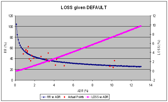
Given current default and recovery rate data, these recovery rate parameters can be easily updated. But on a daily basis, default is not observed in the credit markets for a particular issuer, but loss is. Given risk-free and risky rates, the implied loss rates (aggregate of default and recovery) are known. The following graph plots the study data versus loss (in addition to certain constant recovery rate assumptions).

For investment
grade names (lower loss rates, tighter spreads), a constant recovery rate
assumption of 0.40 is seems to be quite close if nothing else is known. Ideally,
the recovery rate parameters for single name CDSs should reflect company
fundamentals as well as the general economic climate. Intuitively, an
economic climate of high losses (wider spreads) should reduce recovery based solely
upon assets on the balance sheet. (e.g. the same commercial jet has a lower
residual value if other carriers are defaulting or are otherwise uninterested
in purchasing the leftovers). Conversely, an economic climate of low losses
(tighter spreads) should allow the expected recovery derived from the company’s
balance sheet alone to be realized. In their July 2006 paper, “Implied
Recovery”, the authors, Das and Hanouna, skillfully combine elements from both
reduced-form models and structural models to identify recovery rates. As an example of determining the recovery
rate parameters for a single name credit, the following graph and tables show
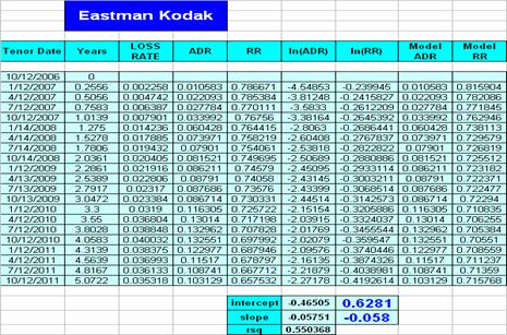
our results for Eastman Kodak (EK) as of day end on
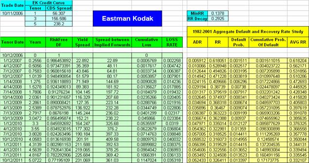
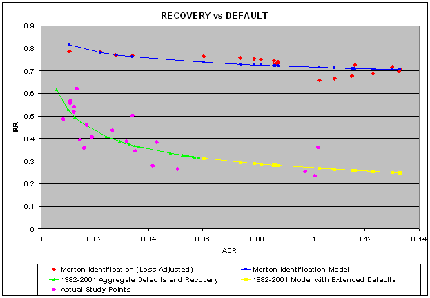
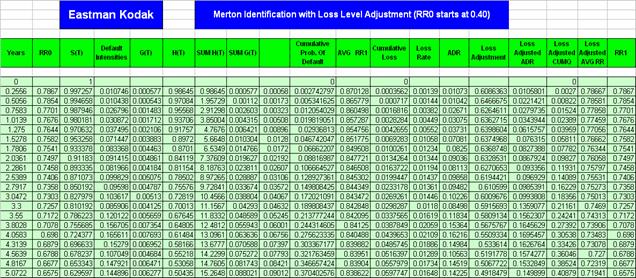
The final table shows the Eastman Kodak minimum recovery rate and decay factor to be 0.628 and 0.0575, respectively. Although the Merton identification approach (as described in the Das and Hanouna paper) converges, it seems to do so at unexpectedly high recovery rates (and therefore unexpectedly high default rates given the same loss level). This happens despite the fact the raw Merton identification function gives very low default rates. The problem appears to come about because the identification function occurs at very low loss levels (minimum loss rate equals 2.205E-16, maximum loss rate is 0.00731) but is applied at much higher loss levels (identification occurs in one domain but is applied to another). Loss levels from the term structure are at much higher levels (minimum loss rate equals 0.00226, maximum loss rate is 0.04). The results shown in the table not only converge via the algorithm but they have been adjusted to the higher loss levels (using default given loss from the raw Merton values). This adjustment brought the recovery rates down, but they still seem higher than expected. We believe these recovery rate levels are not sustainable given an economic downturn and are not consistent with the concerns raised by the Basel II framework document (paragraph 468). The important point here is that you can determine your own recovery rate parameters (given your own judgment and identification methodology) and apply them in the valuation of the CDS. At this time, Kynex is not suggesting what the recovery rate parameters ought to be for a given single name CDS.
Strictly
speaking, every CDS spread in a term structure has an implied recovery rate
associated with it. Given today’s market, that rate is almost always
40%. This associated recovery rate is
the one that should be used for valuation (the valuation will be correct, but
the identification of the underlying probability of default will be off).