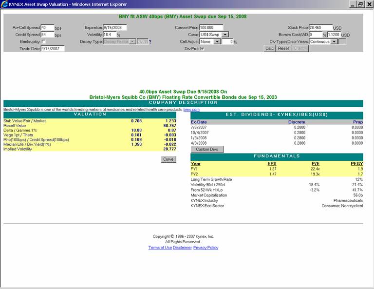
The valuation of an Asset Swap (ASW) on a convertible
security consists of two parts: valuation of the recall value and valuation of
the stub. The latest release of the
Kynex valuation model values the ASW stub as an American style call
option on a convertible bond. The ASW recall value is calculated by our
interest-rate swap calculator, and has not been changed.
Asset Swaps allow an investor to take advantage of the
Gamma of the option embedded in a convertible, while providing insulation against
deterioration of the credit of the issuer. Since entering into an Asset Swap
releases capital, the holder of an Asset Swap can be significantly more levered
than the holder of the underlying bond. This can both magnify the return on the
investment (in favorable circumstances) and lead to a greater negative return
(in unfavorable circumstances).
While we use an American call option framework to
value the ASW stub, it is important to note certain differences between a
simple call option on a stock and a call option on a convertible. An Asset Swap
typically expires on the first call date (or first put date) of a convertible,
i.e. the bond typically does not terminate prior to the expiration of the Asset
Swap. However, we have also observed several examples of Asset Swaps which
expire on the maturity of the underlying bond, even though the bonds are
callable and/or put-able prior to maturity. The model enforces the boundary
condition that if the underlying bond is called (or put) before the expiration
of the Asset Swap, the Asset Swap terminates at the same time that the
underlying bond is terminated. The recall strike of an Asset Swap accretes with
time (reaching par at the expiration of the Asset Swap) i.e. if the stock price
does not change over time, the option goes more out of the money; hence the
time value of an Asset Swap decreases faster than that of a fixed-strike option
(higher negative Theta). This is a subtlety not encountered in pricing standard
equity options. The accreting strike feature is also included in the Kynex
valuation model.
In general, we expect an Asset Swap to be favorable in the
following scenarios:
-
Credit of the issuer of
the convertible deteriorates considerably
-
Interest rates rise
meaningfully
-
Volatility rises
meaningfully and Gamma is realized
-
Desire to not lock-up
capital or hedge fund does not have enough capital
-
Coupon on the convert
is small and recall spread is tight
We also expect an Asset Swap might not be advantageous in
the following scenarios:
-
Recall spread is wide
to begin with and credit tightens considerably
-
Interest rates decline
meaningfully
-
Volatility collapses
and very little Gamma is realized
-
Coupon on the convert
is big and recall spread is wide
We present various scenarios analyzed by us to
quantify the advantages of entering into an Asset Swap vs. holding the
underlying bond.
Scenarios
A few highlights are worth noting before delving into
the details.
- The ASW holder does not receive any coupons but does
not need to finance the “bond” portion that is swapped away. The convertible
holder receives the coupons but has to finance the entire market value of the
convertible. This dynamic affects the cost of carry in a significant way. For
low-coupon convertibles, the ASW holder is not giving up much but the
convertible holder is financing the bond at a much higher rate than the coupon
received. For high-coupon convertibles, the ASW holder is giving up quite a bit
and the convertible holder is able to offset the cost of financing with the
coupons received.
- Since the ASW has a higher negative Theta than the
convertible, the holder of the Asset Swap needs to realize volatility and/or
the interest rates have to rise to overcome the higher rate of time decay.
- If an investor is concerned about the deterioration
of the credit of the issuer, the underlying bond should be valued with our
bankruptcy mode turned on. (The description of the Kynex convertible valuation model
with bankruptcy mode is described in the Dec 2003 Kynex Bulletin.) We analyzed the relative
merits in both modes i.e. bankruptcy mode turned on and off. For the bankruptcy
mode, we employed a decay factor of 1, which means that the credit spread is
expected to double if the stock price declines to half of its current level. When
using the bankruptcy mode, you can set the decay factor to an appropriate level
based on the issuer’s expected creditworthiness, etc. In practice, we found
that the merit of entering into an Asset Swap (as opposed to holding the
underlying bond), does not depend on whether the bankruptcy mode is on or off.
- The Kynex calculator values the underlying
convertible using the risky-risky framework (risky stock growth, risky
discounting of cash flows), and the Asset Swap as risk-free (risk-free stock
growth, risk-free discounting).
The quantitative comparisons were performed using the
Kynex Impact Analysis. The initial position consisted of 1,000 (1 million face)
convertible bonds or Asset Swap on 1,000 bonds. In each case, a short stock
hedge was set up to make the initial portfolio Delta-neutral. A time horizon of
1 yr was employed. The P&L from Gamma trading was calculated using the
Hedge Calculator. For our investigations, we used two example bonds and Asset Swaps:
The first example is a bond with a relatively low
coupon and the Asset Swap has a tight recall spread. We used the AMGN Tranche-1
0.125% 2011 convertible bond. This is a bullet bond. We created an Asset Swap,
whose expiration is equal to the maturity of the bond (Feb 1, 2011), and a recall spread of
30 bps.
The second example is a bond with a higher coupon and
the Asset Swap has a wide recall spread. We used the China Medical (CMED) 3.5%
2011 bond (also a bullet bond). We created an Asset Swap whose expiration is
also equal to the maturity of the bond (Nov 15, 2011), and a recall spread of 300 bps.
We considered two possibilities for our analysis:
The investor enters into an Asset Swap, which releases
capital, thereby making the investor more levered than a bondholder.
The Asset Swap holder invests the released capital at
the risk-free rate. In this scenario, the Asset Swap holder locks up the same
capital (and has effectively the same leverage) as a bondholder.
For each of the above possibilities, we valued the
bond and Asset Swap with the bankruptcy mode turned on and off. Hence there
were a total of four calculations for each scenario. The quantitative results
for the AMGN bond/Asset Swap are summarized in Table 1 and for the CMED bond/Asset Swap in Table 2 (see below).
At the initiation of an Asset Swap, the recall spread
of an Asset Swap is equal to the credit spread of the issuer. In our analysis,
we therefore valued the AMGN bond and ASW with a spread of 30 bps, and the CMED
bond and ASW with a spread of 300 bps. The stock price, bond price, volatility,
credit spread and yield curve, etc., used for our analysis are shown in Table 3 below. Additional pertinent ancillary data are presented
in Tables 4 and 5. Table 4 shows the final bond price, ASW recall value and
stub value for the various scenarios. Table 5 shows the
P&L (from Gamma trading of the stock) and the carry for the bond and ASW. The
carry for the AMGN Asset Swap is substantially higher than for the convertible,
because the bondholder has to finance the bond, and receives little income from
the small coupon. The carry for the CMED Asset Swap is about the same as that
of the convertible because in this case the bondholder receives a substantial
income from the large coupon, which offsets the financing of the bond position.
The ratio of (recall value)/(convertible price) is a
measure of how soon the Asset Swap hits its floor as the credit deteriorates.
The bond price, Asset Swap recall value, and the above ratio are also presented
in Table 3. The value of the ratio is 0.92 for AMGN and
0.76 for CMED. Hence the CMED Asset Swap has a longer way to go to hit the
floor. This means that the CMED Asset Swap has much more negative time decay
than the AMGN Asset Swap. Our analysis illustrates how the larger time decay of
the CMED Asset Swap considerably reduces its rate of return, making it a less
attractive investment compared to the AMGN Asset Swap.
We summarize the results of our study below.
Stock Price, Volatility, Credit Spread, and
Interest Rates are Unchanged
For both AMGN and CMED (with and without the
bankruptcy mode), the underlying bond outperforms the Asset Swap. This can be
attributed to the higher rate of time decay of the Asset Swap relative to its
underlying bond. (Recall that the upward accretion of the strike price with
time causes an Asset Swap to go out of the money if all other parameters remain
constant.) Basically, if volatility is not realized and/or interest rates do
not increase, then an Asset Swap is not advantageous.
Stock Price
Falls, Credit Spread Widens, and Implied
Volatility Increases
We expect that a fall in the stock price may be
correlated with a deterioration of the credit of the issuer (i.e. wider credit
spread). The volatility may also typically increase. The widening of the credit
spread and increase in the implied volatility are offsetting factors with
respect to the change in the value of the Asset Swap.
The AMGN Asset Swap outperformed the underlying bond.
The CMED Asset Swap underperformed relative to the
underlying bond. This was traced to the effect on carry (as described earlier)
due to the high coupon as well as the distance between the market price and the
ASW recall value. The increase in the
implied volatility helps the Asset Swap holder, but (in the case of CMED) not
by enough to outperform the bondholder. Both the AMGN and CMED Asset Swaps hit
their respective floors in this scenario. For AMGN the floor is 87.0. The
initial market price is 90, so the ASW investor suffers a loss of 3.0 before
the floor kicks in. For CMED the floor is 85.4. The initial market price is 107,
so the investor suffers a loss of 21.6 points before the floor kicks in. An Asset
Swap investor is only protected against a widening of the credit spread after
the floor is reached. Hence an investor holding the CMED Asset Swap loses
substantial value if the spread widens, before the protection of the Asset Swap
takes effect.
The above statements were made assuming that the Asset
Swap investor is more highly levered than the bondholder. If the Asset Swap
holder has the same capital as the bondholder, and invests the extra capital at
the risk free rate, then in both examples the Asset Swap holder receives a
better return than the bondholder.
The use of the bankruptcy mode changes the
quantitative numbers but does not alter the above conclusions.
Stock Price
Rises, Credit Spread Tightens, and Implied Volatility Decreases
We might expect that the results will be the opposite
of the previous scenario. Both the AMGN and CMED Asset Swaps under-perform
compared to their underlying bonds. The magnitude of the under-performance of
the CMED Asset swap is much more than that of the AMGN. This is due to the
effect on the carry (as described earlier) due to the higher coupon on the CMED
convertible. The above statements assume that the Asset Swap investor is more
highly levered than the bondholder. If the Asset Swap holder has the same
capital as the bondholder, and invests the extra capital at the risk free rate,
then the magnitude of under-performance of the Asset Swap is lesser.
The use of the bankruptcy mode changes the
quantitative numbers but not the relative performances of the bonds and Asset
Swaps.
Interest
Rates Rise/Fall 100 bps
We hold the stock price etc., fixed in the Impact
Analysis, but apply an impact of a 100bp rise/fall (parallel shift) in the
interest rates. We expect that if interest rates rise, the Asset Swap
outperforms the bond, and if interest rates fall, the Asset Swap will give a
lower rate of return than the underlying bond.
Our findings do not completely confirm this
expectation. For the AMGN bond and Asset Swap, the above behavior is observed
(with both the bankruptcy mode on and off). The CMED Asset Swap, however,
underperforms the bond even when interest
rates rise, when the bankruptcy mode is off. This is again due to the
effect on carry due to the high coupon as well as the longer distance between
the market price and the ASW re-call value. When the bankruptcy mode is on, the
CMED Asset Swap outperforms the underlying bond when the interest rates rise.
The CMED Asset Swap underperforms the bond when the interest rates fall, both
with and without the bankruptcy mode on.
The above statements assume that the Asset Swap
investor is more levered than the bondholder. If the Asset Swap holder has the
same capital as the bondholder (and invests the extra capital at the risk-free
rate), then the return obtained by the Asset Swap holder might or might not be
better than the bondholder when interest rates rise (both with and without the
bankruptcy mode) depending on other factors such as carry, theta, etc.
The above findings for CMED are consistent with our
expectation that an Asset Swap is not advantageous if the bond pays a large
coupon and has a wide spread to begin with.
Credit
Default Swap (CDS)
Another possibility for the investor to hedge against deterioration
in the credit of the issuer is to buy protection via a Credit Default Swap
(CDS). Please refer to our December
2006 Bulletin for more details. In this
scenario, the investor holds the underlying convertible bond, and therefore
does not unlock any capital. The CDS requires deal payments, which can drag
down the return on the portfolio. The CDS reduces the required short stock
position to be Delta-neutral since the CDS provides a hedge against credit
deterioration which is correlated with stock price declines (most of the time),
so in our analysis below we employed a lighter stock hedge.
We considered an example CDS on the AMGN Tranche 1
bond. The deal spread on the CDS is 30 bps (equal to the recall spread of the Asset
Swap). The CDS maturity was set to March 20, 2011 (with a first coupon date of June 20, 2007). From Table 3, the hedge Delta of the bond is 48. We set the CDS
notional to hedge 8%, and hedged the remaining 40% with a short stock position.
The return on the bond + CDS + short stock position was calculated for a
horizon of 1 year (the same as with the Asset Swap). Table 6
shows the return on the CDS (with a stock hedge of 40%, as noted above). The
corresponding return obtained by using an Asset Swap (with a stock hedge of
48%) is also shown. The data for the Asset Swap was copied from Table 1 (the data where the bankruptcy mode was turned on).
The returns are presented for the two scenarios
·
stock price declines, spreads rise, implied
volatility increases
·
stock price rises, spreads tighten, implied
volatility decreases
Note that the bankruptcy mode must be turned on when
valuing the bond (the use of a CDS implies a probability of default). Recall
that we set the decay factor to 1. We see from Table 6 that
the use of a CDS (and light short stock position) does not give as good a
return as the use of an Asset Swap in the first scenario (stock price declines
and the spread widens). The CDS gives a better return than an Asset Swap when
the stock price increases and the spreads tighten. This is because, in this
scenario, the Asset Swap suffers from the reduction in the realized volatility and has large time decay. The bond + CDS
portfolio does not have such large time decay.
For reference, we also constructed a CDS on the CMED
bond, and display the results in Table 6. The deal
spread on the CDS is 300 bps (equal to the recall spread of the Asset Swap).
The CDS maturity was set to Dec
20, 2011 (with a first coupon date of June 20, 2007). For CMED, we already know that
the convertible bond by itself (with Delta-neutral short stock hedge)
outperforms the Asset Swap in both cases when the stock falls and credit widens
and the stock rises and credit tightens. The use of a CDS (with a light stock
hedge of 60 instead of 68) also outperforms the Asset Swap in both of the above
scenarios.
However, there are other factors to consider when
deciding to hedge with a CDS or to enter into an Asset Swap. There is no
clear-cut best solution. Some points to note are:
A CDS is more liquid than an Asset Swap. Furthermore,
the bond and CDS trade independently, so it is easier for the investor to
change the position in the bond and/or CDS.
An Asset Swap holder is essentially locked into the
position until the expiration (or recall) of the Asset Swap. To change the
position, the investor must buy new convertibles and enter into a new Asset
Swap agreement with a broker.
A CDS does not release capital, whereas an Asset Swap
does. A hedge fund with limited capital may have no choice but to enter into an
Asset Swap.
Metrics
We compare various metrics of an Asset Swap vs. the
underlying bond below. For example, Asset Swaps usually have a lower Delta than
the underlying bond, and are therefore hedged using a smaller short stock
position. Furthermore the value of Rho
is negative for a convertible bond, but is positive for an Asset Swap. Hence an
Asset Swap has an implicit hedge against a rise in interest rates, as we noted
in the Impact Analysis study above.
We performed sweeps with the bankruptcy mode off and
also with the bankruptcy mode on. With the bankruptcy mode off, we used the
AMGN bond and Asset Swap mentioned above. We performed four sets of sweeps
(Spot price, Volatility, Credit Spread and an Interest Rate Shift (parallel
shift of yield curve)). The graphs are shown in Figures 1
through 28 below. With the bankruptcy mode on, we employed
the CMED bond and Asset Swap mentioned above. The graphs are shown in Figures 29 through 36 below.
Bankruptcy
Mode Off
We discuss the case of bankruptcy mode on below, after
first analyzing the results for the case of bankruptcy mode off. The input
parameters for the AMGN bond and Asset Swap are the same as in Table 3, except for the credit spread. If an Asset Swap is
valued by setting the credit spread of the underlying bond equal to the ASW
recall spread, then we have found that the median life of the Asset Swap is
zero. The advantage of entering into an Asset Swap is based on the expectation
of the future credit spreads, behavior of the volatility and interest rates
etc. For the purposes of comparison of the bond and Asset Swap metrics, we
valued the AMGN bond with a credit spread of 150 bps.
We swept the stock price, volatility, credit spread
and interest rates. For each sweep, we plotted graphs of the bond fair value
and Asset Swap stub fair value, Delta, Gamma, Vega, Rho, Credit Spread 01, Theta and the median life.
In all the graphs, the dark blue curve describes the bond and the pink curve
describes the Asset Swap. We analyze the comparison of the metrics below.
Stock Sweep
The graphs
obtained by sweeping the stock price are the most informative of the various
sweeps.
·
The first graph displays the bond fair value and
Asset Swap stub as a function of the stock price. As expected, they both have a
(smoothed out) hockey stick shape.
·
The graph of Delta indicates that the Asset Swap
has a lower Delta than the bond. This is consistent with the market expectation
that holding an Asset Swap requires a smaller hedge than holding a bond.
·
The Gamma of the Asset Swap has a peak which is
slightly higher than the bond, and the location of the peak is also slightly
displaced to a higher stock price. At about S=110, the two graphs coincide. At
this stock price level, the median life of the Asset Swap decreases to zero,
and so the Gamma of the Asset Swap equals that of the bond.
·
The Vega curve is similar to the Gamma curve.
·
The graph of Rho shows a significant difference in the
behavior of the Asset Swap and the bond. The curves are parallel, but Rho is positive for the Asset
Swap and negative for the bond. This is indicative of the fact that the Asset
Swap holder is not exposed to the interest rate sensitivity of the “pure bond”
part of the convertible (which is negative).
·
The graph of the credit spread01 sensitivity
also shows a significant difference in the behavior of the Asset Swap and the
bond. The curve for the bond is negative. The curve for the Asset Swap is
almost zero, indicative of the fact that the Asset Swap holder has divested himself
of the credit risk of the issuer.
·
The graph of Theta shows that the Asset Swap has
more negative time decay than the underlying bond. Roughly speaking, the pure
bond part of the convertible has a positive Theta (accretion to par), and the
option part has a negative Theta. The Asset Swap holder has only the option
part. Effectively, the Asset Swap holder has removed the exposure to the credit
risk of the issuer, but at the price of more negative time decay.
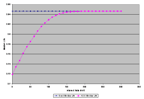
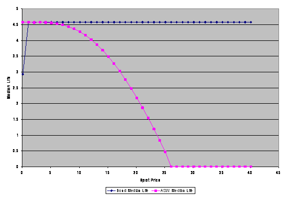
·
The median life of the bond is always equal to
the time to maturity, since this is a bullet bond. The median life of the Asset
Swap is also equal to the time to maturity at low stock prices, but then
decreases with increasing stock price and drops to zero above about S=110. At
such high values of S, the sensitivity to credit spread is very small, and the
expected value of the cash flows including the value of the option embedded in the
bond make it preferable to hold the convertible.
Volatility Sweep
The graphs
obtained by sweeping the volatility are mostly featureless, and are included
for completeness of the presentation. The median life of the Asset Swap
displays a complicated dependence on the volatility, but it is difficult to
draw any conclusions from this fact.
Credit Spread Sweep
The graphs
obtained by sweeping the credit spread illustrate one fairly obvious point. In
all the plots, the curve for the Asset Swap becomes flat as the credit spread
is increased. This is consistent with our expectation that, at high spreads,
the bond value declines and contributes little to the valuation of the Asset
Swap. (Think of a deep out of the money option.) The Asset Swap (which is
valued on a risk-free basis) is then insensitive to the precise value of the
credit spread, leading to flat curves in the plots.
Interest Rate Shift
Unlike a sweep of the
credit spread, an interest rate shift changes the risk-free interest rate. This
affects the recall value of the Asset Swap, whereas a change in the credit
spread does not. The curves for the Asset Swap therefore do not flatten out as
the risk-free rate increases. The graph of the Asset Swap stub and bond fair
value is the most informative. Since the Asset Swap has a positive Rho and the bond has a negative Rho, the ASW stub value and the bond fair
value move in opposite directions as the risk-free rate increases.
Bankruptcy Mode On
We now discuss
the case of bankruptcy mode on. As stated above, we employ the CMED bond and
Asset Swap. The parameters are the same as in Table 3. We
swept only the stock price. We know that when the bankruptcy mode is on, at low
parity the fair value of the bond drops to zero, the bond Delta increases (in
principle to infinity at zero parity), and the Gamma is negative. However, the
Asset Swap stub value has a floor of zero and the Delta and Gamma behave more
like those of an equity call option, i.e. Delta increases from 0 and 100 in an
S-curve as the stock price increases, and Gamma is always positive. Hence we
expect a significant difference in the graphs of the bond and the Asset Swap.
This is confirmed in Figures 29 through 36 below. We again plotted graphs of the bond fair
value and Asset Swap stub fair value, Delta, Gamma, Vega, Rho, Credit Spread 01, Theta and the median life.
In all the graphs, the dark blue curve again describes the bond and the pink
curve describes the Asset Swap.
We see that the median life of the Asset
Swap drops to zero at about S=26. The interesting behavior is when the Asset
Swap median life is nonzero, i.e. S<26. As the parity decreases to zero, the
holder of an Asset Swap would decrease the stock hedge to zero, whereas a
bondholder would need to increase the stock hedge. Furthermore, the bondholder
would be hurt by the negative Gamma, but an Asset Swap holder does not have
this problem. Furthermore, even in the region where both the bond and Asset
Swap have positive Gamma (e.g. S=24, which is the stock price used in the
scenario analysis above), the Asset Swap has substantially more Gamma than the
bond. This explains why, in Table 5,
the P&L for the CMED Asset Swap, with bankruptcy mode on, is substantially
larger than the P&L for the underlying convertible.
The graph for Rho (Figure 33)
indicates that the Asset Swap continues to have an implicit hedge against a
rise in interest rates, and the graph for Theta (Figure
35) indicates that the Asset Swap
continues to have more negative time decay than the underlying bond. Switching
on the bankruptcy mode does not change these aspects of the behavior of an
Asset Swap.
The graphs for the AMGN Asset Swap and bond,
with the bankruptcy mode on, are similar but the differences are not as
pronounced. Basically, with the bankruptcy mode on, if the median life of the
Asset Swap is nonzero, then the Asset Swap has a substantially larger Gamma
than the underlying convertible, as well as a smaller Delta (which goes to zero
whereas the bond Delta goes to infinity at zero parity). The Asset Swap holder
can realize much greater P&L from Gamma trading.
Table 1 – Return on Bond and Asset Swap for AMGN Tranche 1
|
Scenario
|
Bankruptcy Mode Off
|
Bankruptcy Mode On
|
|
Bond
|
ASW
|
Bond
|
ASW
|
|
No excess capital
|
Invest excess
capital at risk-free rate
|
No excess capital
|
Invest excess
capital at risk-free rate
|
|
Return
|
P&L($)
|
Return
|
P&L($)
|
Return
|
P&L($)
|
Return
|
P&L($)
|
Return
|
P&L($)
|
Return
|
P&L($)
|
|
Unchanged
|
5.33%
|
11,990
|
3.23%
|
610
|
4.85%
|
10,917
|
5.14%
|
11,576
|
0.97%
|
182
|
4.66%
|
10,489
|
|
Interest Rates Rise 100 bps
|
– 2.17%
|
–4,890
|
37.02%
|
7,020
|
7.70%
|
17,322
|
–2.33%
|
–5,234
|
35.20%
|
6,677
|
7.55%
|
16,978
|
|
Interest Rates Fall 100 bps
|
13.32%
|
29,970
|
–28.95%
|
–5,489
|
2.14%
|
4,812
|
13.09%
|
29,446
|
–31.36%
|
–5961
|
1.93%
|
4,338
|
|
Stock Down 20%, Spread Widens, Implied Volatility Increases
|
–0.70%
|
–1,586
|
137.15%
|
25,953
|
16.11%
|
36,257
|
–6.70%
|
–15,070
|
134.75%
|
25,499
|
15.91%
|
35,803
|
|
Stock Up 20%, Spread Tightens, Implied Volatility Decreases
|
–2.25%
|
–5,054
|
–87.79%
|
–16,398
|
–2.70%
|
–6,082
|
–2.18%
|
–4,908
|
–86.90%
|
–16481
|
–2.75%
|
–6,180
|
Table
2 – Return on Bond and Asset Swap for CMED
|
Scenario
|
Bankruptcy Mode Off
|
Bankruptcy Mode On
|
|
Bond
|
ASW
|
Bond
|
ASW
|
|
No excess capital
|
Invest excess
capital at risk-free rate
|
No excess capital
|
Invest excess
capital at risk-free rate
|
|
Return
|
P&L($)
|
Return
|
P&L($)
|
Return
|
P&L($)
|
Return
|
P&L($)
|
Return
|
P&L($)
|
Return
|
P&L($)
|
|
Unchanged
|
8.95%
|
23,935
|
–23.58%
|
–15,029
|
–1.81%
|
–4,840
|
6.83%
|
18,723
|
–2.79%
|
–1,776
|
3.14%
|
8,412
|
|
Interest Rates Rise 100 bps
|
2.17%
|
5,795
|
–6.40%
|
–4,080
|
2.28%
|
6,109
|
0.56%
|
1,493
|
16.58%
|
10,562
|
7.76%
|
20,751
|
|
Interest Rates Fall 100 bps
|
16.19%
|
43,295
|
–40.68%
|
–25,923
|
–5.88%
|
–15,734
|
13.47%
|
36,033
|
–22.40%
|
–14,270
|
–1.53%
|
–4,081
|
|
Stock Down 20%, Spread Widens, Implied Volatility Increases
|
–88.54%
|
–236,846
|
–183.78%
|
–117,150
|
–39.99%
|
–106,962
|
–95.3%
|
–254,798
|
–171.4%
|
–109,268
|
–37.04%
|
–99,080
|
|
Stock Up 20%, Spread Tightens, Implied Volatility Decreases
|
2.16%
|
5,765
|
–52.81%
|
–33,649
|
–8.77%
|
–23,460
|
5.33%
|
14,263
|
–9.08%
|
–5787
|
1.65%
|
4,402
|
Table 3 – Input Parameters for P&L and Impact Analysis
|
Parameter
|
AMGN
|
CMED
|
|
Bond Price
|
90
|
107
|
|
ASW Recall Value
|
82.45
|
81.51
|
|
Recall Value/Bond Price
|
0.92
|
0.76
|
|
Stock Price
|
60
|
24
|
|
Volatility
|
19
|
35
|
|
Credit Spread (bps)
|
30
|
300
|
|
Yield Curve
|
US $Swap
|
US $Swap
|
|
Borrow Cost
|
0
|
0
|
|
Dividend Model
|
Continuous
|
Continuous
|
|
Bond/ASW Quantity
|
1000
|
1000
|
|
Delta Hedge
|
48
|
68
|
|
Finance/Rebate Rate
|
5.75/5.00
|
5.75/5.00
|
|
Horizon
|
1 year
|
1 year
|
|
Leverage
|
4
|
4
|
|
Bond Capital ($)
|
225,000
|
267,500
|
|
ASW Capital ($)
|
18,877
|
63,727
|
|
ASW Leverage if no excel capital
|
47.7
|
16.8
|
Table 4
– Bond Price and ASW Recall Value & Stub Value
|
Scenario
|
AMGN
|
CMED
|
|
Bond Price
|
ASW
|
Bond Price
|
ASW
|
|
Recall Value
|
Stub Value
|
Recall Value
|
Stub Value
|
|
Initial
|
90
|
82.45
|
7.55
|
107
|
81.51
|
25.49
|
|
Interest Rates
Rise 100 bps
|
90.0
|
84.66
|
5.34
|
103.93
|
82.52
|
21.41
|
|
Interest Rates
Fall 100 bps
|
93.48
|
89.39
|
4.08
|
107.69
|
88.45
|
19.24
|
|
Stock Down
20%, Spread Widens, Implied Volatility Increases
|
83.12
|
87.01
|
0
|
69.55
|
85.42
|
0
|
|
Stock Up 20%,
Spread Tightens, Implied Volatility Decreases
|
97.20
|
87.33
|
9.87
|
114.02
|
85.43
|
28.60
|
Table 5 – Gamma Trading P&L and Carry for Bond & ASW
|
Scenario
|
AMGN
|
CMED
|
|
Bond
|
ASW
|
Bond
|
ASW
|
|
P&L Bankruptcy
Mode Off
|
14,680
|
14,680
|
22,147
|
22,147
|
|
P&L Bankruptcy
Mode On
|
14,226
|
14,226
|
11,115
|
30,029
|
|
Carry
|
–19,580
|
14,828
|
14,218
|
14,396
|
Table 6 – Return on Portfolio using CDS or Asset Swap
|
Scenario
|
AMGN
|
CMED
|
|
Bond + CDS + light hedge
|
ASW (from table 1)
|
Bond + CDS + light hedge
|
ASW (from Table 2)
|
|
No excess capital
|
Invest excess capital at risk-free rate
|
No excess capital
|
Invest excess capital at risk-free rate
|
|
Stock Down 20%, Spread
Widens, Implied Volatility Increases
|
10.22%
|
134.75%
|
15.91%
|
–92.5%
|
–171.41%
|
–37.04%
|
|
Stock Up 20%, Spread
Tightens, Implied Volatility Decreases
|
–3.58%
|
–83.33%
|
–2.65%
|
4.94%
|
–9.08%
|
1.65%
|
AMGN Tranche-1 Bond & ASW valued with CS = 150 bps
Figure 1 Bond Fair Value & ASW Stub v. Spot Price
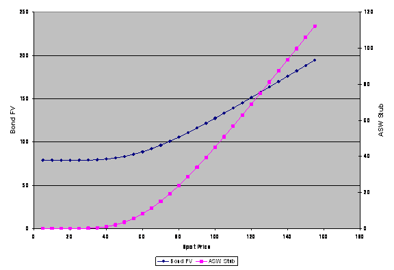
Figure 2 Bond & ASW Delta v. Spot
Price
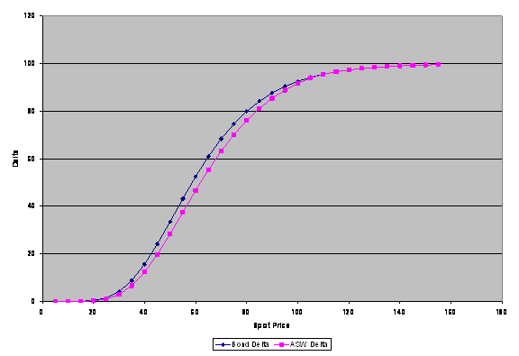
Figure 3 Bond & ASW Gamma v. Spot
Price
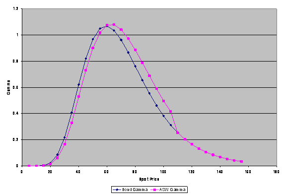
Figure 4 Bond & ASW Vega v. Spot Price
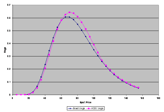
Figure 5 Bond & ASW Rho v. Spot Price
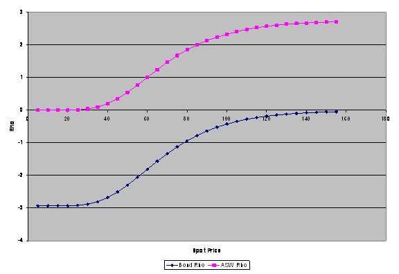
Figure 6 Bond & ASW Credit Spread01 v.
Spot Price
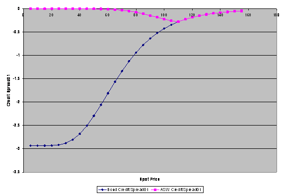
Figure 7 Bond & ASW Theta v. Spot
Price
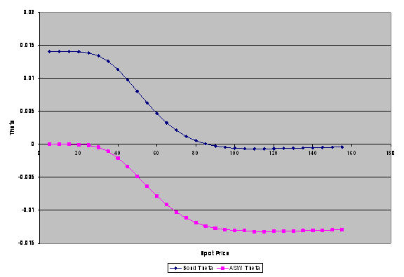
Figure 8 Bond & ASW Median Life v.
Spot Price
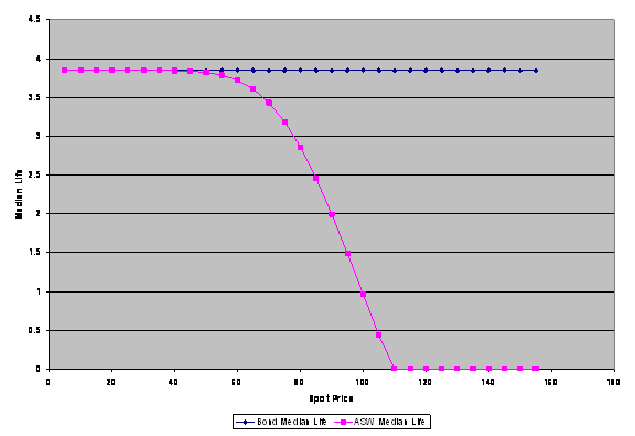
Figure 9 Bond Fair Value & ASW Stub v.
Volatility
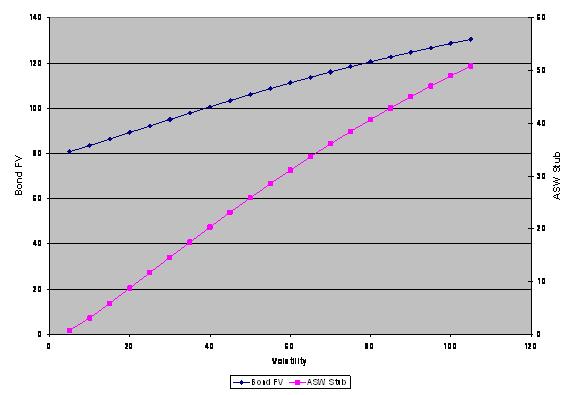
Figure 10 Bond & ASW Delta v. Volatility
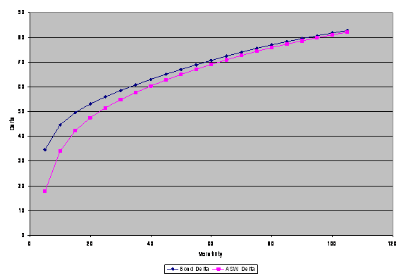
Figure 11 Bond & ASW Gamma v. Volatility
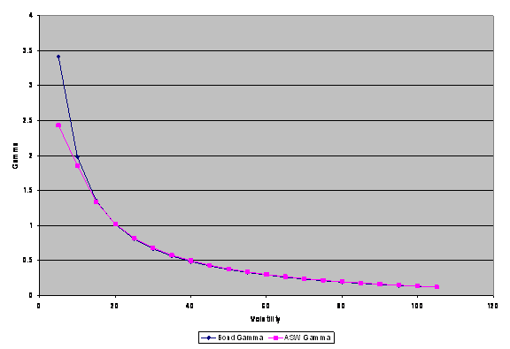
Figure 12 Bond & ASW Vega v. Volatility
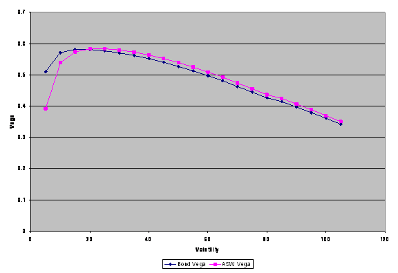
Figure 13 Bond & ASW Rho v. Volatility
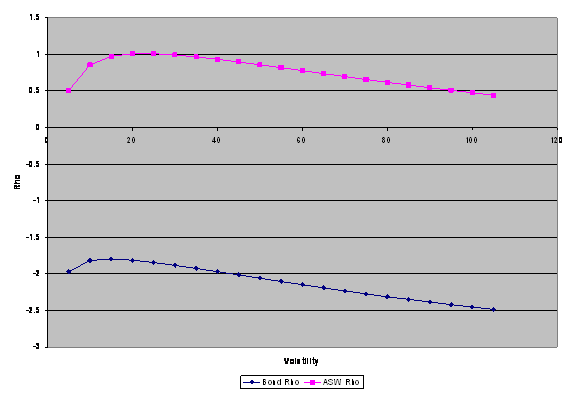
Figure 14 Bond & ASW Credit Spread01
v. Volatility
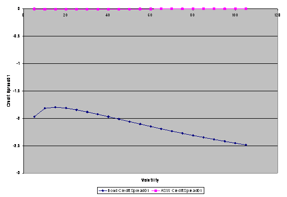
Figure 15 Bond & ASW Theta v. Volatility
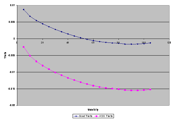
Figure 16 Bond & ASW Median Life v. Volatility
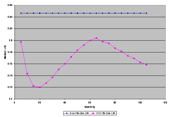
Figure 17 Bond Fair Value & ASW Stub v.
Credit Spread
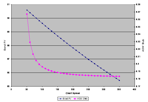
Figure 18 Bond & ASW Delta v. Credit
Spread
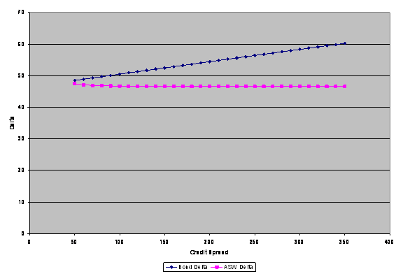
Figure 19 Bond & ASW Gamma v. Credit
Spread
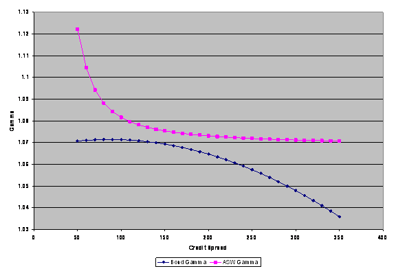
Figure 20 Bond & ASW Vega v. Credit
Spread
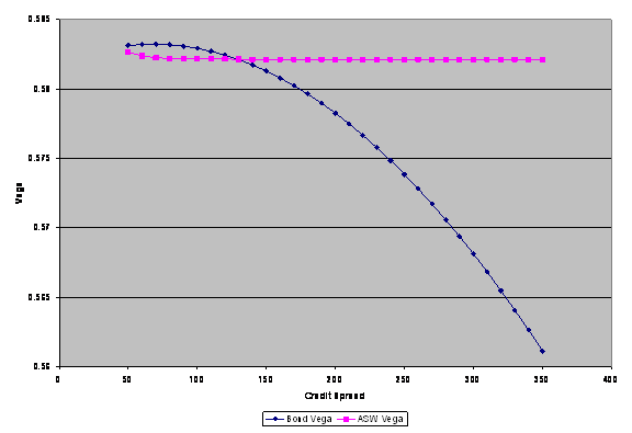
Figure 21 Bond & ASW Theta v. Credit
Spread
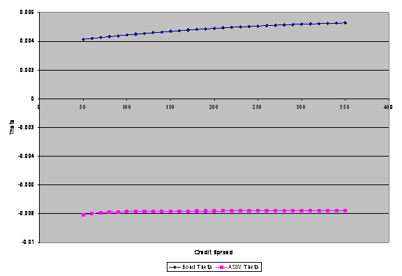
Figure 22 Bond & ASW Median Life v. Credit
Spread
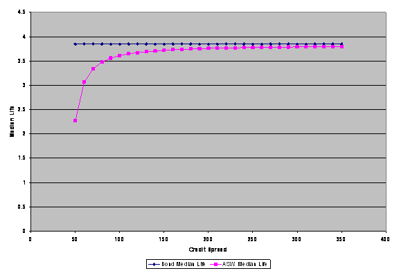
Figure 23 Bond Fair Value & ASW Stub
v. Interest Rate Shift
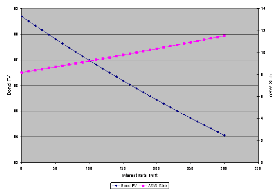
Figure 24 Bond & ASW Delta v. Interest
Rate Shift
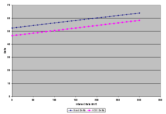
Figure 25 Bond & ASW Gamma v. Interest
Rate Shift
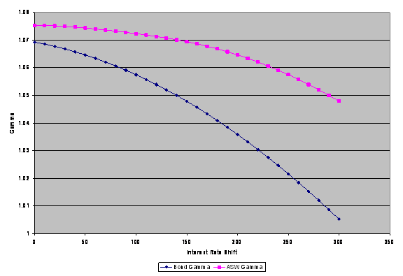
Figure 26 Bond & ASW Vega v. Interest
Rate Shift
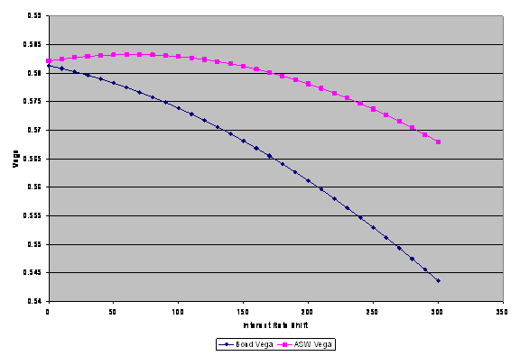
Figure 27 Bond & ASW Theta v. Interest
Rate Shift
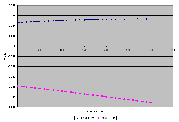
Figure 28 Bond & ASW Median Life v. Interest Rate Shift
CMED Bond & ASW valued with bankruptcy mode on
Figure 29 Bond Fair Value & ASW Stub v. Spot Price (CMED,
bankruptcy mode on)
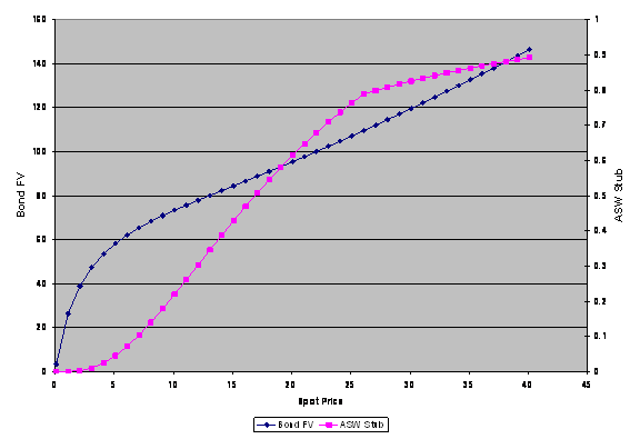
Figure 30 CMED Bond & ASW Delta v. Spot
Price (CMED, bankruptcy mode on)
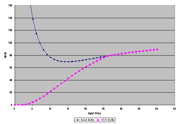
Figure 31 CMED Bond & ASW Gamma v. Spot
Price (CMED, bankruptcy mode on)
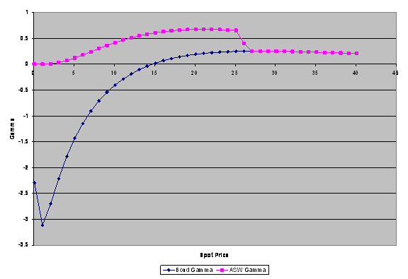
Figure 32 CMED Bond & ASW Vega v. Spot
Price (CMED, bankruptcy mode on)
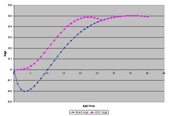
Figure 33 CMED Bond & ASW Rho
v. Spot Price (CMED, bankruptcy mode on)
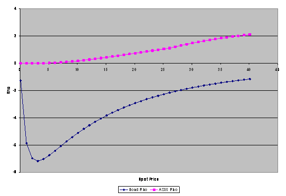
Figure 34 CMED Bond & ASW Credit
Sperad01 v. Spot Price (CMED, bankruptcy mode on)
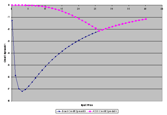
Figure 35 CMED Bond & ASW Theta v. Spot Price (CMED, bankruptcy
mode on)
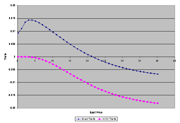
Figure 36 CMED Bond & ASW Median Life v. Spot Price (CMED,
bankruptcy mode on)
Top