Kynex Interest Rate Shift Methodology
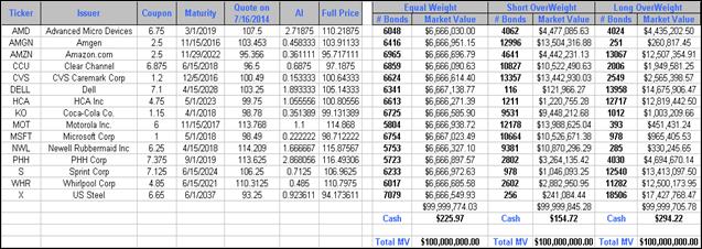
To illustrate the desirability of and the need for our methodology, we constructed three portfolios. These portfolios can be found in the Appendix. All three portfolios contain the same fifteen corporate bonds chosen by us to span the duration spectrum and the credit spectrum. The notional amounts of each bond in the three portfolios are different, but each portfolio has a starting market value of $100 million. In the first portfolio, the notional amounts are equal weighted in market value dollars. In the second portfolio the notional amounts are adjusted such that the shorter duration bonds are overweight relative to intermediate and longer duration bonds. In the third portfolio the notional amounts are adjusted such that the longer duration bonds are overweight relative to shorter duration bonds.
We ran four scenarios of yield curve shifts and corresponding spread shifts. The results and our analysis follow.
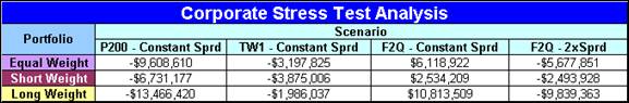
The first scenario is a parallel upward shift of 200 basis points of the yield curve (P200) and the credit spreads are held at the same level as they were before the shift. This is the most common and simple scenario that we have observed run on several desks. As depicted in the chart, the long-weighted portfolio suffers the most loss and the short-weighted portfolio suffers the least. This relationship between portfolios holds for any possible parallel shift.
Our observation of past history suggests yield curves rarely shift in a parallel manner. In the current environment, a more likely scenario when the Federal Reserve starts to raise rates is an upward and flattening shift to the yield curve. The second scenario shifts the 2-year rate up by 200 basis points, 10-year rate by 25 basis points and the 30-year rate remains unchanged (TW1). Credit spreads remain constant. We fit the rest of the curve using our twist method to generate a realistic curve with smooth forwards. As shown in the chart, the long-weighted portfolio suffers the least and the short-weighted portfolio suffers the most. This is the exact opposite of the result from the first scenario and the magnitude of losses is also significantly different. The point is that a portfolio’s change in market value cannot be reduced to some combination of parallel shifts. Twists are necessary to fully capture possible rate changes in the market. In our opinion, the twist tool generated non-parallel shift in the yield curve provides a more realistic alternative to the more usual means of adjusting curves. Please see a more detailed discussion below.
The third scenario attempts to simulate a flight to quality where rates at every tenor are cut in half thereby lowering and steepening the curve (F2Q). While the shift in the yield curve is non-parallel, we held the credit spreads at the same level as they were before the shift. As you can see in the chart, all three portfolios gain in value. Obviously, this credit spread assumption is incompatible with the benchmark shift assumed for a flight to quality scenario. These calculations are meaningless.
In the fourth scenario, a flight to quality is once again assumed. The yield curve is shifted in the same way as in the third scenario. However the credit spreads on individual bonds are doubled from where they were before the shifts were applied – bonds with a spread of 50 bps go to 100 bps and bonds with 200 bps go to 400 bps. This captures what we have observed in the market when there is a flight to quality. All corporate bonds sell off but the magnitude of the sell-off is more severe in the high-yield spectrum relative to high-grade spectrum, i.e. CCC and B rated bonds suffer more than A and AA rated bonds. As presented in the chart, all three portfolios now lose in value and the long-weighted portfolio suffers a bigger loss than the short-weighted portfolio. This outcome is more realistic and observed in the past during a market flight-to-quality period.
A portfolio’s rate and spread risk evaluation should include some use of parallel shifts. But the exclusive use of parallel shifts is a mistake. We recommend the inclusion of non-parallel shifts to the yield curve and corresponding shifts of bond credit spreads depending on the kind of market stress that you want captured. Blindly calculating all possible combinations of benchmark shifts and credit shifts may lead to the inclusion of meaningless results.
One of the benefits of subscribing to our portfolio
analytics is the ability to create and run stress tests. Our stress tests give you the ability to move
equity prices, volatility, credit spreads, interest rates or any combinations
of these factors with the goal of quantifying the risk/reward to your portfolio
given hypothetical market scenarios. We
currently have 3 canned scenarios which are available
to all of our clients (Kynex Stress Test,
Interest Rate Stress Test
and 2008 Stress Test). If you’d like to create your own custom
stress test you are able to do so as well.
If you are not familiar with this feature or are interested in trialing
the portfolio/stress test, please contact us at 201-796-4900.
In terms of benchmark movements, our stress tests
provide the same flexibility as our Yield Curve Analysis Tool. Most
importantly, we recognize that parallel shifts rarely occur in the market. In
most cases, yield curves are twisting to some extent. For example in our 2008
Stress test we simulate the market transition from the 3rd Quarter
of 2008 prior to the Lehman default to the end of the 1st Quarter of
2009 in which the S&P declined 39%.
During this time period, the 2 year point tightened 57% (186bps), the 10
year point tightened 35% (153bps) and the 30 year point tightened 32% (150bps).
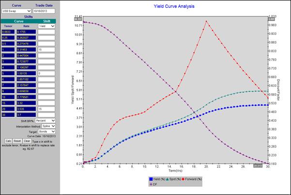
The blue line indicates the
In our 2008 Stress Test, we use percentage movements
as opposed to basis points. We will
illustrate why this is important.
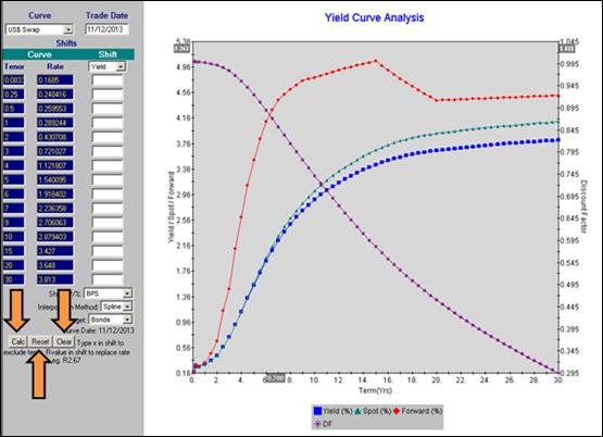
Please find below the October 30, 2013 curve (blue)
and the same curve adjusted using a BPS shift from the 2008-2009 Interest Rate
Environment (IRE) (red). Given the low
rates today, a shift of the same basis point maginitude puts the entire front
end of the curve at zero thus producing a nonsensical curve. For this reason, we recommend using
percentage movements in these scenarios.
For more detail on bps vs. percentage adjustments, please see the Appendix.
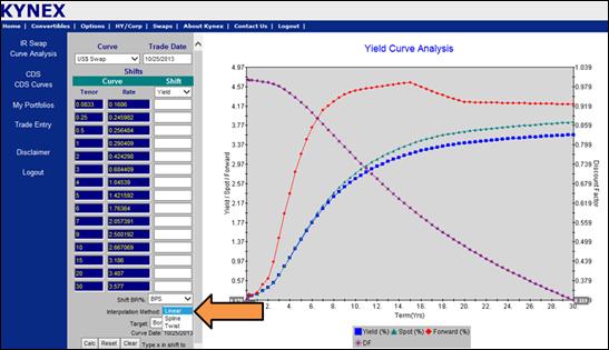
You can choose to use a Linear, Spline, or Twist
interpolation method for our stress tests.
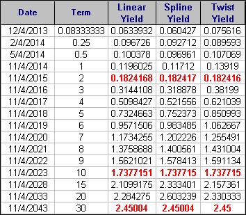
Once again, please consider the October 30, 2013 US$Swap curve. The
tables and graph below show a comparison of the three interpolation methods
using our 2008 Stress Test parameters.
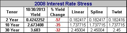
Regardless
of the interpolation method, the yields of the specified tenors match. The Linear and Spline will follow the curve but will
produce different yields for the intermediate points. The Kynex Twist is not
constrained by the existing curve. It attempts to assign yields that will
simplify the forward rate structure. Because of this, the forward rates remain
well-behaved whenever possible.
Although the yield curves appear close, the forward
rate structure of each method is quite different. Please find the graphical
comparison of the forward rate structures below.
In this case, the Twist assumption gives a more
reasonable approximation of the adjusted yield curve because its forward rate
structure does not have the additional complexity in the other two. Often, the
points on the existing curve will skew the adjustment you are trying to apply.
If you assume that the 2 year, the 10 year and the 30 year rates are moving,
you would reasonably assume that other points on the curve are moving as well.
A shock to a single rate just does not happen in the market, and risk assessment
assuming this can be misleading. The
resulting adjusted curve from a Twist is intended as a curve which could exist
in the market while still hitting the rates pegged at the specified tenors.
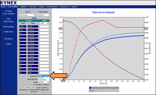
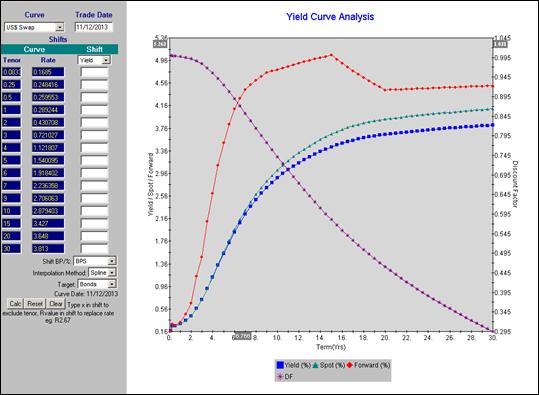
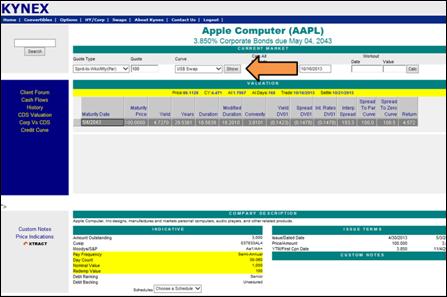
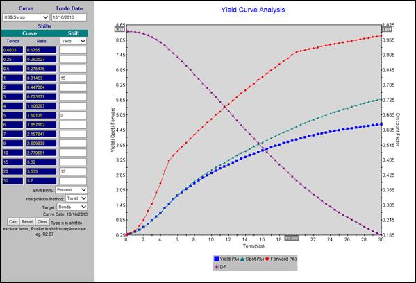
Before
trying to adjust your benchmark curve, it is important to know what the Yield
Curve Analysis actually shows. You can
navigate to the Yield Curve Analysis by going to Swaps and then Curve
Analysis. From here, Kynex
defaults to the
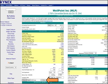
OR
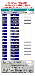
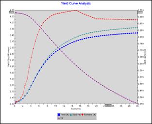
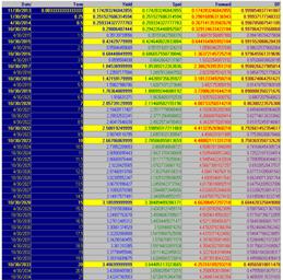
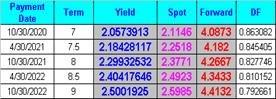
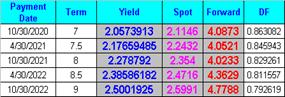
From the main valuation details page you can navigate to the designated native curve by pressing Show. Once Analyze is pressed, the native rates (along with the underlying source parameters that fully define each rate) are used to calculate the full IRE. IRE consists of yields, spots and forward rates which will give identical discount factors when applied. Forward rates (red line on the graph and red numerals in the table) are derived using the Kynex forward rate model. This model connects and smoothes the forward rates while maintaining term structure as well as no arbitrage on the yields. All values (e.g. yields and spots) derived at intermediate tenors are calculated from the forwards. Additional information on this bootstrap process can be found in the Interest Rate Swaps article in the December 2003 Kynex Bulletin.
Direct interpolation on yields and spots is never done. Interpolation directly on yields destroys the existing forward rate structure. An example is shown in the Appendix to illustrate (along with a brief discussion of splits).
The forward rates help you to see even the smallest inconsistency in the rates of the native yield curve tenors vis-à-vis the other tenor values. Note that an inconsistency is not necessarily wrong. An example of this inconsistency can be seen on the long end of the 10/25/2013 US$ Swap Curve. As we noted in the 9/12/2012 Kynex Flash Bulletin, the front end of our swap curve is calculated using the Euro-Dollar contracts. But the long end tenors (15, 20 and 30 year tenors) come from the swap market. These two markets are obviously related. They trade closely, but they are separate markets. This small difference can be seen in the forward rate starting 15 years out. This 15 year “hump” can be caused by the slight inconsistency between the 10 year Euro-Dollar contract and that of the swap market. The swap market will also have some liquidity issues at the long end. In this case, the Euro-Dollar contracts suggest a 10 year swap yield of 2.667069 while the swap market comes in at 2.667. This suggests that the 15 year and the 20 year swap rates are slightly awry. You can correct for the 15 year in two ways. You can remove the 15 year tenor by entering an “X” next to the rate. This will remove that tenor from the bootstrap. Note that the forward rate model corrects the 15 year yield from 3.186 to 3.164.
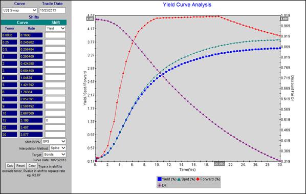
This new yield is consistent with the 10 year yield and the 20 year yield. You can replace the 15 year tenor by entering an “R” followed by a value. If you enter “R3.164”, you will get the same IRE.
Mixing securities with different liquidities into one benchmark curve is neither necessary nor desirable. More tenors do not necessarily give more accuracy. More gives less accuracy if unlike securities are scrambled together.
Kynex does not offer an On/Off-the-Run curve for a reason.
A well-known and popular data and analytics vendor does, however. We took those
Treasury securities constituting its On/Off-the-Run Curve and priced all
Treasuries using end-of-day prices from TreasuryDirect (https://www.treasurydirect.gov/GA-FI/FedInvest/selectSecurityPriceDate.htm) for 10/22/2013. The resulting On/Off-the-Run Curve as well
as an On-the-Run Curve is shown
below.
Ostensibly, the reason usually given for using the On/Off-the-Run Curve is to give additional curvature on the yield curve for those maturities not covered by the currents. The two IRE’s clearly show this is not the case. In fact, only noise is introduced by mixing unlike securities. Off-the-Runs will almost always trade at a higher yield. For example, 912828TS9 (T 0.625% 9/30/2017) and 912810FP8 (T 5.375% 2/15/2031) are two of the Off-the-Runs mixed with the currents in the above example. If 912828TS9 was priced as a current, its yield would be 4.65 basis points lower, and 912810FP8 would have a lower yield by 6.18 basis points.
Benchmark Curve Adjustment Mechanics
There
are three basic steps that you need to take before making a benchmark
adjustment. The first step is
determining what you want to adjust. The
Kynex Yield Curve Analysis gives you the ability to specify your changes to the
Yields, Spots
or Forwards.

Second, you must specify how the adjustment will be applied. You can specify adjustments in basis points added to the curve (BPS). Percent adjustments are interpreted as a percentage movement to the benchmark value. If you know your new value, you can also specify that value as a Target Rate.
Next you need to select your Interpolation Method. Kynex currently supports three Shift Interpolation Methods: Linear, Spline, and Twist. Each is briefly described below.
Linear Method
Values at intermediate terms are interpolated linearly between consecutive specified tenors.
Spline Method
The Spline Interpolation method requires a minimum of three spreads, and we use a piecewise quadratic interpolation method for the intermediate values.
Unlike, the linear and spline method, the Twist method does not follow the existing curve
at all the tenors. Rather, the twist will hit the specified tenor values (if possible), but the twist model is free to assign realistic values at the intermediate points. You will see below that abrupt adjustments using the spline and linear methods can result in IREs which could never happen in the real world.
Finally, you can apply your shift by selecting Calc. This action will capture your adjustments and return the resulting yields, spots and forwards. If at any time you wish to clear your adjustment and restore the default benchmark curve, you can do so by selecting Clear. If you are in the midst of making changes and would like to restore the adjustment that was made the last time you selected Calc, you can do so by selecting Reset.
The
Kynex Yield Curve Analysis will show you the result of your desired adjustment.
Often, you may get what you expect. When more complicated adjustments are
desired, you may get a surprise. For example, consider the IRE for the
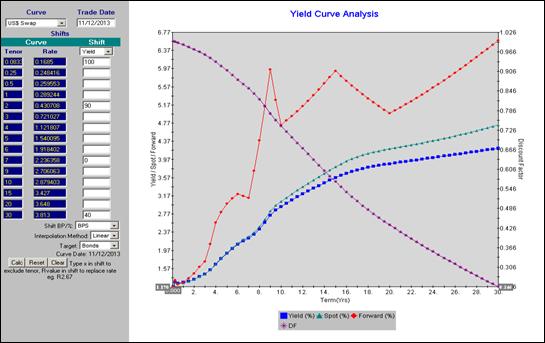
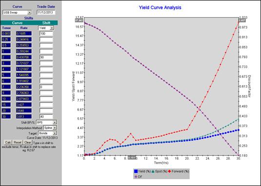
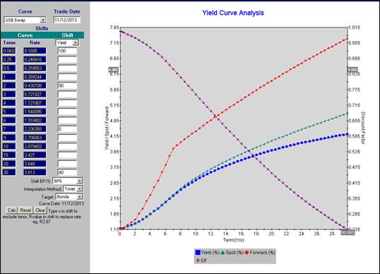
Consider a yield adjustment of 100bps on the one month tenor, 90bps on the 2 year tenor, 0bps at the 7 year tenor, and 40bps at the 30year tenor. The resulting IREs for each of the interpolation types are shown below.
Linear Adjustment
Spline Adjustment
Kynex Twist
US$ Swap curves corresponding to the linear and
spline adjustment will never happen in the real market. The yields are
inconsistent. The Kynex Twist gives a
plausible curve that still satisfies the designated yields at the specified
tenors. All three yield curves are plotted below.
Note that the Kynex Twist generally gives the simplest and most direct solution to the designated pegs on the curve. The point here is not to suggest the exclusive use of the Twist adjustment. We do recommend that you do not blindly make curve adjustments. Please check the implications of your rate adjustments. The Kynex Yield Curve Analysis allows you to do this easily.
Benchmark Curve Adjustment for a Specific Bond
Using
AAPL 3.85% Corporate Bonds due May 2043, we illustrate a parallel shift, a butterfly
shift, and a twist. Assume this bond is priced at 100bps over swaps for a price
of 86.1128 on 10/16/2013. Select the Show button next to
the curve label. This should pop up the designated curve. On that window, the
adjustments can be entered. Additional specifics on these Examples can be found
in the Appendix.
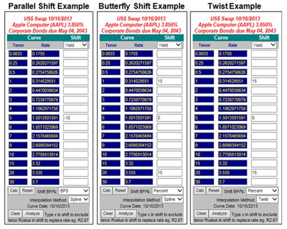
As you would expect the price for the simple downward parallel shift of 10bps increases to 87.6106. In the butterfly and twist examples, we mimic short term and long term rates increasing at a greater magnitude than the medium term rates. But the results are different. In the butterfly example, the price falls to 71.9886. The price given the Twist scenario is slightly higher at 72.2406. You must press Analyze to determine this difference. Even though yields at the pegs are satisfied, the IREs are quite different.
For the Butterfly Shift Example, percentage changes to yields have been specified at the tenors. The corresponding spline (please see the Appendix for details) somewhat unexpectedly results in yield decreases for the 10 year and 15 year tenors (real world concerns will never intrude upon a spline’s mindless mathematics). The resulting IRE is graphed below.
Butterfly
Shift Example
Applying the same adjustment values but using instead a Twist method rather than a Spline, we obtain a much smoother curve and something more realistically observable in the market. In this Twist Example, forwards as well as yields are modeled. For example, the yield on the 10 year tenor does decrease, but by only 5 bps. The yield on the 15 year tenor increases by almost 20 bps. Ultimately, these rates are converted to discount factors on the dates of the bond’s cash flows, and these flows are discounted to settlement to arrive at the full price of the bond.
Twist
Example
Kynex has always had several ways to apply credit adjustments in order to properly measure a bond’s credit quality and subordination. We will consider the discount factor and default probability consequences for each of the various types of adjustments. Depending upon how you arrive at the proper credit adjustment, one way may be more appropriate or useful than another. Please consider AMD 6.75% Corporate Bond due March 2019. We assume that it trades at 106.75 on 6/10/2014.
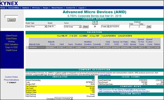
The interpolated spread is the traditional way of measuring the bond price versus its future cash flows. It is a yield spread measure. It assumes the risk free rate is constant (for every cash flow) and equal to the yield on the risk free curve at the same point as the redemption date (in this case, the maturity date) of the bond. The quoted spread to a specific Treasury bond is yet another variation of a yield spread. The par spread measure recognizes that benchmark yields are not constant. They have a term structure. As such risky discount factors for earlier cash flows are different from those for later cash flows. The par spread is a parallel shift in bps on the benchmark yields which equates the present value of future flows with the full price of the bond. The zero spread is similar to the par spread except that it is a parallel shift in bps in benchmark spot rates which equates the present value of future flows with the full price of the bond. The zero spread and par spread are equivalent (but not numerically equal) only if the benchmark yields and their corresponding spots are arbitrage free. The discount factors and cumulative probability of defaults are shown below for each of these three measures. The Kynex Default Probability Model is discussed in the December 2006 Kynex Bulletin. We have assumed a constant 39% recovery rate for all AMD default calculations. As you can see, the default probability path is not substantially different for these three types of constant spreads. A detailed discussion of spread types can be found below.
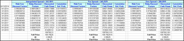
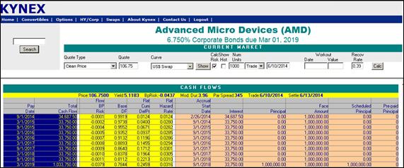
Regardless of the type of quote on a bond, Kynex will always show the default path of the corresponding flat par spread on the Cash Flow analytic Please see below.
But we know that credit spreads are not constant in the market. The CDS credit curve for AMD is shown below.
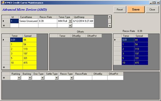
These
CDS par spreads can be used to calculate a cumulative default probability path.
The price of any AMD bond with the same subordination should be consistent with
this default path. But an issuer my have older bonds as well as new issues. Depending upon the coupons, some bonds will be priced at par while others are
priced at a premium or discount. The Kynex tool that allows an analyst to price
any issuer’s bond with equal subordination is the Corp vs CDS analytic. Consider the newly issued
AMD bond with a coupon of 7% and maturing on 7/1/2024. On 6/10/2014, this bond
traded at 102.50. At that price, the market assumed that the bond should trade
to the 7/1/2022 call date.
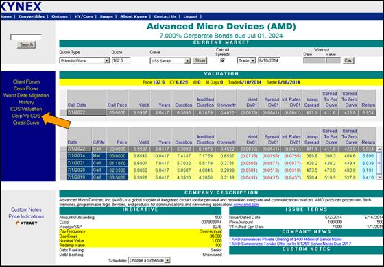
Kynex tracks the average funding in the market for a 5 year CDS. On 6/10/2014, this funding value was 44bps over three-month Libor. The resulting Corp vs CDS analytic is shown below.
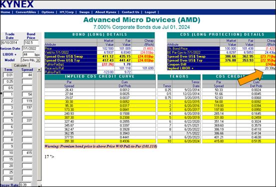
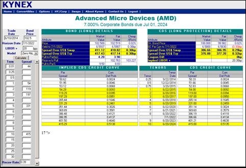
Our models that price bonds using a CDS credit curve are extensively discussed in the July 2009 Kynex Bulletin. The 44 bps funding assumption shows a dislocation between the bond and the CDS. But this assumption is an average one, and it is calculated from five year bonds. This analytic suggests that the proper funding for AMD is 20bps over Libor. As shown below, the dislocation is eliminated at 20bps. The model price of 102.52 almost agrees with the market price.
We then apply these same CDS parameters to AMD 6.75%
3/1/2019.
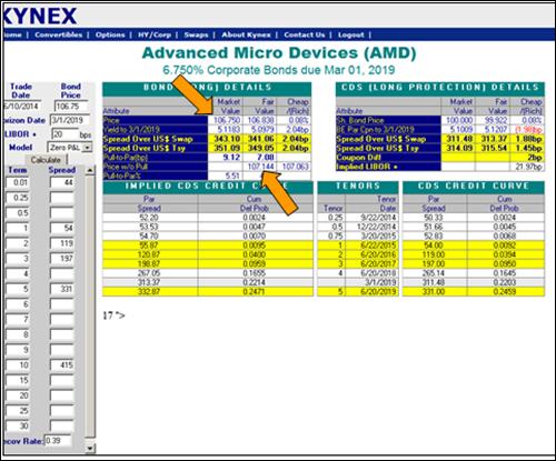
Again, no dislocation exists. The CDS fair value of the bond (106.838) is well within the bid-ask market price (106.75). The default probability path is almost identical for both bonds. Note that the fair value of the bond is not equal to the risky present value (107.144) of its cash flows. AMD 6.75% 3/1/2019 is a premium bond. It has more to lose if default occurs than a par bond (with a coupon at around 5.1%) or a discount bond. The Kynex Pull-to-Par Model and the Zero P&L Basis Trade Model account for this additional loss on premium bonds (or gain on discount bonds). This is a critical difference between a CDS spread (which is always at par) and a credit spread. The two are numerically equal (approximately) only for par bonds. A further discussion of spreads can be found below.
The
relationship can be clearly seen by looking at default probability paths.
Consider the AMD 6.75% 3/1/2019 bond as we did in the above example. We have used
the curvature from the CDS credit curve to create a spread term structure which
identically prices the cash flows.
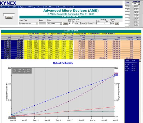
The
flat cumulative default probability path is as before. The term structure
probability path increases and requires more default by maturity. The flat path
has almost identical hazard rates, while the hazard rates corresponding to that
of the term structure increase. For normally shaped credit curves, a flat
spread quote will overestimate the default probability path for the early dates
and underestimate values for the later dates. It is instructive to compare all default paths together. As expected, the spreads and the default paths
are higher for the AMD premium bond.
They
reflect the price of the bond in the market. That price reflects the additional
loss for premium bonds with higher coupons. The CDS credit curve and its
default path reflects the underlying default for the issuer if it were to issue
par bonds. The CDS credit curve is a measure of the credit worthiness of the
issuer. Bond discount factors must reflect this and the additional aspects
(e.g. coupon, subordination, funding, and liquidity) in the bond market.
Flat
credit spreads applied to longer bonds and perpetual preferred stock can be
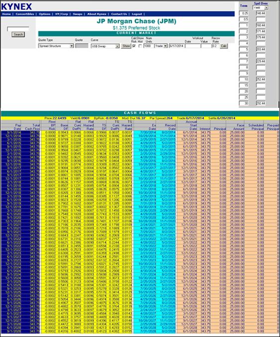
misleading, especially for wide spreads. Consider the JPM $1.375 preferred
stock trading at 22.65 on 6/17/2014. For perpetuals, we calculate yields for
infinite cash flows even though we specify a maturity date of 100 years beyond
the next dividend date (9/1/2114).
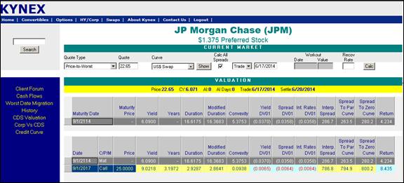
This is used for the presentation of cash flows seen below.
Due to lack of space, we have continued the table below. We have also specified a spread term structure which is consistent with the CDS credit curve as well as pricing the bond identically at 22.65.
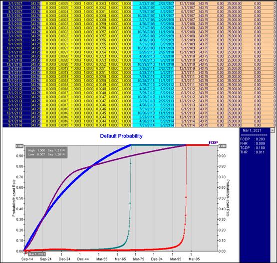
Please note that the corresponding default paths for the flat spread versus the term structure are significantly different. But both measures have default paths that suggest this perpetual will eventually default. For the flat spread, default occurs by 9/1/2072. For the spread term structure assumption, default occurs by 9/1/2102. If spreads are assumed to be wider, default will occur much sooner. If the recovery rate is higher, default will also occur much sooner. If we had assumed a recovery rate of 40% rather than 20% (and using the same spreads), the default for the flat spread is certain by 9/1/2047 (just over 33 years). For the term structure, default occurs by 3/1/2042 (not even 28 years). Please see the corresponding default paths based upon a 40% recovery.
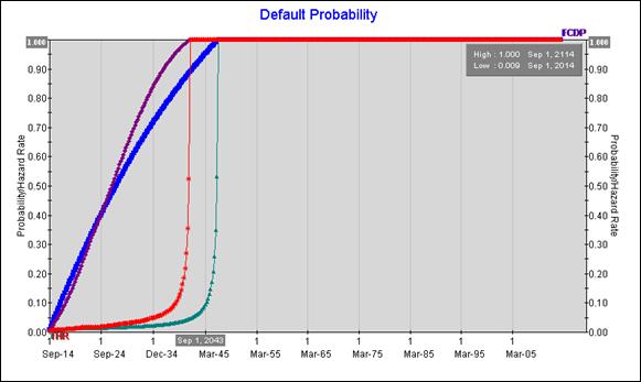
Kynex
uses these results to justify ending the convertible grid after 30 years.
Benchmark
Yield Curves and Credit Spreads
Every convertible bond or corporate bond valuation begins
with the benchmark curve bootstrap. The bootstrap’s purpose is to identify
risk-free rates (or the least risky) across the whole spectrum of maturities.
The tenor rates on the curve are assumed to be homogenous. They have identical
credit worthiness and liquidity. Because of this assumption, one can
legitimately calculate the intermediate spot rates and forward rates for any
point on the curve. The more sophisticated bootstraps usually control the
implied forwards being calculated. Kynex uses its own Forward Rate Model to
accomplish this calculation. As a result, the Kynex forward rates accurately measure the change in rates over time only. Therefore, these rates can be used to value
interest rate swaps or project coupon rates on floating rate bonds. An
important part of the Kynex bootstrap is a method which optimally handles
shocks at various points on the curve.
Prior to the development of the more sophisticated
bootstrap methods, unlike securities were mixed together to form a single yield
curve. Historically, this has taken the form of so called On/Off-the-Run curves
in which currents are mixed with older Treasuries ostensibly to obtain more
curvature. Kynex does not support these
curves for several reasons. First, our Forward Rate Model already models the
amount of curvature as well as concavity. As we demonstrate elsewhere, mixing unlike securities here only creates noise from the
difference in liquidity. The resulting forward rates are a hodge-podge mixture
of liquidity change and time-to-maturity change.
An important part of the Kynex Yield Curve Analysis is the ability to adjust benchmark curves in various ways. A full discussion of these adjustments is found above. Kynex allows you to adjust the curve by specifying adjustments at certain tenors. These adjustments are then used by the specified interpolation method to apply these changes to the rest of the tenors on the curve. The linear and the spline interpolation types will follow the existing shape of the curve. These more usual ways of adjusting yields can lead to curves whose forward rate structure is unrealistic. They would never happen in the market. The Kynex Twist is designed to hit the desired tenor values while still maintaining a realistic forward rate structure. We provide several specific examples above.
The corporate bond market has
evolved several different measures for quantifying the credit worthiness of a
bond issue. Before the advent of interest rate swaps in the early 1980’s,
corporate bonds were usually quoted by a broker as a spread to a particular
Treasury bond. This spread was merely added to the yield of that Treasury.
Since this Treasury bond usually traded far more frequently than the corporate,
this broker quote became established as the usual form for pricing the
corporate bond. It was easy to determine the bond price even though the
corporate was not trading. So long as the corporate market moved with the
Treasury market, this quoting method remained robust.
But all brokers (especially those with a large Government
desk) recognized that the equilibrium between the corporate market and the
Treasury market was not static. Even if we ignore large disruptions (e.g. a
flight to quality) in which these markets move in opposite directions, broker
quotes are far from ideal. That single benchmark Treasury may have started off
being a current, but it soon becomes an off-the-run with less liquidity
vis-à-vis the new currents. The corporate bond based upon that Treasury would
require either a spread change or a benchmark change. If current Treasury rates
drop, the older Treasury necessarily becomes a premium bond whose yields will
go up but at a decreasing rate. This Pull-to-Par is documented in the May 2008 Kynex
Bulletin.
Any coupon difference between the corporate bond and the Treasury bond
will only increase the price tracking differences between the two.
For other spread products (e.g. mortgage pass-thrus, agency
CMO’s), the broker requirement to price using only currents can cause a
maturity mismatch. A 4 year bond might
be priced over the 3/5 split. This would mean the spread would be added to the
average yield on the 3 year Treasury current with that of the 5 year Treasury
current. This type of broker quote would obviously underestimate the yield on a true 4 year Treasury bond if it were to be auctioned
(assuming a normally shaped yield curve). As in the case of a split quote, the
interpolated spread was introduced as a way of eliminating a maturity mismatch.
However, this type of quote is normally associated with an interpolation
directly on yields. It has the same problems as quotes based upon splits.
However, with the introduction of sophisticated bootstrap methods, the usual
problems with this quote are eliminated. Kynex uses its own Forward Rate Model
to identify yields at any point on a yield curve that is precisely consistent
with term structure. Kynex never interpolates directly on yields. These yields
are displayed in tabular and graphical format by the Curve
Analysis link. Please see the first page
for the link location.
Even with the Kynex bootstrap, the interpolated spread is
still only a yield based measure. Certainly, a bond’s cash flows occur at many
points over the entire curve. The interpolated spread only measures to a single
redemption point. The Kynex par spread
is a spread over the whole curve. Its corresponding discount factors are based
upon many rates, not just a single yield. Simply stated, the par spread is the
basis point parallel shift over benchmark yields required to make the bond’s full
price equal to the discounted value of its cash flows. Similarly, the zero
spread is defined as the basis point shift over benchmark spot rates required
to equate the bond full price with its discounted cash flows. The Kynex Forward
Rate Model ensures that the spot curve and the yield curve are equivalent (not
numerically equal). This equivalence ensures that the two curves have identical
discount factors at every point.
Over time, benchmark curves rarely move in parallel. Kynex
allows benchmark yields and spots to be adjusted differently at each tenor.
However, not every tenor needs to be specified. Kynex has several interpolation
types to “fill” between the adjusted tenors. Please see above for a more detailed discussion.
Corporate bonds can also be valued using CDS spreads and
credit curves. Although a CDS spread and a credit spread are numerically equal
(approximately) for a bond priced at par, it is important to understand the
difference between the two. The credit spread of a bond captures all the
factors determining the price of the bond.
That certainly includes the probability of default by the issuer and any
recovery value. But it includes so much more. Maybe the bond has embedded call
options, thus widening the credit spread. Maybe the bond has a very large
coupon or a very small coupon verses what would be normally offered in the
current market. The credit spread would be larger or smaller based upon the
corresponding price compression. Maybe this bond is thinly traded. Maybe it has
a difference in tax treatment. Maybe this bond is subordinated in its company’s
capital structure. The point here is that the CDS spread measures the
likelihood of the issuer’s default, not the probability of a bond’s default or
downgrade.
A CDS spread equates the expected present values of the two
legs of a swap having contingent cash flows. The expected payments leg is paid
by the buyer if default does not occur. The seller of the swap receives the
payments and only pays the notional amount of the insurance (less the recovery
value) if default does occur. The risky discount factors are determined using
the Kynex Default Probability Model discussed in the Appendix of the December 2006
Kynex Bulletin.
If you have a CDS credit curve for an issuer, you can price
any of its fixed-coupon corporate bonds using that credit curve and the Kynex
“Corp vs CDS” analytic. You can maintain wider spreads for subordinated bonds
as part of the credit curve which will automatically be applied. These spreads
can take the form of separate curves or a series of basis point offsets to the
senior curve. You have the choice of two
models: the Kynex Pull-to-Par Model and the Zero P&L Basis Trade Model.
These models are thoroughly discussed in the July 2009 Kynex
Bulletin and the May 2008 Kynex
Bulletin. Both of these models allow the
identification of the market’s funding between bonds and CDS’s. The dislocation
between the corporate bond market and the CDS market is well documented. If a
dislocation exists for a specific bond, this analytic will quantify its
magnitude. It shows the fair value of
the bond assuming the specified CDS credit curve and the funding assumption. It
also displays the implied credit curve or the implied funding assuming the
specified bond price is accurate.
Appendix
Portfolios Used to Illustrate the Kynex
Methodology
Direct
Interpolation on Yields: An Example
0n 10/25/2013, the IRE can be seen below. The forward rate model assigned a yield of 2.299325 at the 8 year point. If we do a linear interpolation directly on yields, the 8 year tenor would have a yield of 2.278792. If that 8 year point is included in the bootstrap, you can clearly see that the linearly interpolated value at the 8 year point is inconsistent with the yields at the 7 and 9 year tenors.
So what? If you are selling, it is beneficial to you to quote off of a split for a normally shaped yield curve. If you are buying, you can use this tool to adjust the spread to compensate for the lower benchmark yield. Either way, you can accurately quantify the spread. In this case, this difference is worth about 5/32nds for an 8 year par security. You can take it or leave it.
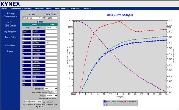
Basis Points vs. Percentage Movements
As mentioned in Benchmark Curve Adjustment Mechanics, you can make adjustments in basis points, percentages, and target rates. Generally, the recommended method is using percentage movements. Using basis point shifts and ignoring how this affects the curve can cause spurious results. For example, below we illustrate the curve on 10/16/2013 with a parallel downward shift of 50 bps. While a 50 bps shift downward may have been a relatively small change 5 or 6 years ago, given today’s interest rate environment it is a huge adjustment. As you can see, the rates are so low at the front of the curve on 10/16/2013 that a shift downward of 50 bps shift puts them at zero. By using percentage movements, you can avoid this problem.
AAPL 3.85% Corporate Bonds due May 2043
AAPL
3.85% Corporate Bonds due May 2043